At this point we’ve developed a good sense of the technical theory of causal reinforcement learning. This next section brings together many important ideas and generalises notions of data transfer between different environments. This will prove important when we discuss imitation learning in the future. For those coming from a more pure reinforcement learning background, being able to generalise results about where and when we can transfer knowledge between related domains is clearly useful for a general agent. Let’s get going!

Generalisability and Robustness

One of the most important features of human intelligence is its ability to generalise and transfer causal knowledge across seemingly disparate domains. This allows powerful inferences and decision making procedures possible even in foreign environments. Bareinboim and Pearl address the problem of transferring knowledge from data collected in heterogeneous domains $\Pi = \{ \pi_1,\dots,\pi_n\}$ to some target domain $\pi^\ast$ - a problem known as $mz$-transportability. In ¹Bareinboim, E., & Pearl, J. (2014). Transportability from multiple environments with limited experiments: Completeness results. NIPS. the authors establish a necessary and sufficient condition for deciding whether this transfer is feasible. In the sciences, powerful studies involving transfer of knowledge across related domains are known as meta-analysis or externally valid studies. The transfer of causal knowledge is known as transportability and is a crucial ability needed for artificial agents to automate the process of knowledge acquisition, discovery and learning.

Consider an example in which we would like to use knowledge of social science experiments done in Los Angeles (predicting outcome $Y$ with cause $X$, confounded by some age distribution $Z$) to make similar predictions in New York. Calling the distribution in Los Angeles $P(y \mid do(x))$, we would like to predict $R = P^\ast(y \mid do(x))$ - the cause/effect relationship under a different age distribution in New York. We call the process which generates this difference in age across the populations a difference generating factor, denoted graphically by $\blacksquare$, which are caused by some set of selection variables $S$. In this case we have $S \rightarrow Z$. We can then derive an remarkably simple transport formula as follows:

$R = \sum_s P^\ast(y \mid do(x), z) P^\ast(z) = \sum_s P(y \mid do(x), z) P^\ast(z)$

This deceptively simple formula tells us we can estimate $R$ - an interventional quantity - using a drop in observational distribution $P^\ast(z \mid do(x), z)$. This acts to re-weight observations by the interventional affect in a different domain. To generalise a transport formula is not completely trivial. We need to know whether $do$-calculus is complete. That is, whether $do$-calculus operations can always find such a transport formula. Recall that causal models and induced diagrams encode relationships under a particular domain. A formalism that is helpful for the study of transfer of knowledge across causal domains is the notion of selection diagrams. These diagrams graphically encode the shared causal relations and difference generating factors of different causal systems.

Selection Diagrams ¹Bareinboim, E., & Pearl, J. (2014). Transportability from multiple environments with limited experiments: Completeness results. NIPS.: Let $\langle M, M^\ast \rangle$ be a pair of structural causal models from domains $\langle \pi, \pi^\ast \rangle$, sharing causal diagram $G$. The pair $\langle M, M^\ast \rangle$ induces a selection diagram $D$ if $D$ obeys the following criteria: (1) every edge in G is also an edge in D, and (2) D contains an extra edge $S_i \rightarrow V_i$ whenever there might exist some discrepancy $f_i \neq f_i^\ast$ or $P(U_i) \neq P^\ast(U_i)$ between $M$ and $M^\ast$.

These $S$ variables in the selection diagram serve as identifying the mechanisms where structural differences in the data generating process takes place between models under different domains. Knowledge of these structural overlaps of different causal domains allows us to formalise what it means to transfer knowledge between domains. This is the notion of $mz$-transportability discussed earlier. Simply put, knowledge is transferable between domains only if the causal effect $R$ can be determined from information available in the observational and interventional distributions.

$mz$-Transportability ¹Bareinboim, E., & Pearl, J. (2014). Transportability from multiple environments with limited experiments: Completeness results. NIPS.: Let $\mathcal{D} = \{ D^{(1)}, \dots, D^{(n)} \}$ be a collection of selection diagrams with source domains $\Pi = \{ \pi_1,\dots,\pi_n \}$ and target domain $\pi^\ast$. Let $\boldsymbol{Z}_i$ be the variables in which experiments can be conducted in domain $\pi_i$. If $\langle P^i, I_z^i \rangle$ are the observational and interventional distributions, then the causal effect $R = P_{\boldsymbol{x}}^\ast (\boldsymbol{y})$ is said to be $mz$-transportable from $\Pi$ to $\pi^\ast$ in $\mathcal{D}$ if $P_{\boldsymbol{x}}^\ast(\boldsymbol{y})$ is uniquely computable from $\cup_{i=1,\dots,n} \langle P^i, I_z^i \rangle \cup \langle P^\ast, I_z^\ast \rangle$ in any model that induces $\mathcal{D}$.

The above graphical condition has a counterpart that can be written in terms of $do$-calculus criteria.

Theorem: Let symbols be defined as above. The effect $R = P^{\ast} (\boldsymbol{y} \mid do(x))$ is $mz$-transportable from $\Pi$ to $\pi^\ast$ if the expression $P(\boldsymbol{y} \mid do(x), \boldsymbol{S}_1, \dots, \boldsymbol{S}_n)$ is reducible using the rules of $do$-calculus to an expression in which (1) do-operators that apply to subsets o $I_z^i$ have no $\boldsymbol{S}_i$-variables or (2) do-operators apply only to subsets of $I_z^i$.

This theorem tells us that do-calculus is complete in terms of finding these transport formulae. The authors also prove completeness for an established algorithm for computing transport formulae. Refer to source material ¹Bareinboim, E., & Pearl, J. (2014). Transportability from multiple environments with limited experiments: Completeness results. NIPS. for details of this algorithm.

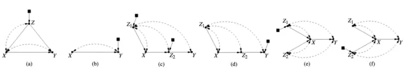
Figures (a) through (f) show illustrative examples of transportability in causal selection diagrams. These highlight the important of the nature of unobserved confounders. (a) This diagram shows an example of when transportability of $R=P^\ast(y \mid do(x))$ is trivially solved by re-weighting of the variable directly affected by difference-generating variable. In this case $S \rightarrow Z$. (b) shows the simplest example in which one cannot transport a causal relation between domains. Even by randomisation on $X$, the causal effect is not uniquely computable due to UCs. (c) and (d) show examples where transportability of causal effects require interventional information over $Z_1$ in $\pi_1$ and $Z_2$ in $\pi_2$, but not over $\{Z_1,Z_2\}$ in the combined domain. (e) and (f) show examples where transportability is only possible in the combined domain. Figure extracted from ¹Bareinboim, E., & Pearl, J. (2014). Transportability from multiple environments with limited experiments: Completeness results. NIPS..

This process of transferring knowledge relates well to the concept of unifying big data. The ability to fuse multiple datasets, collected under heterogeneous conditions, without incurring large bias penalties is something critically important for generalising an agent’s ability to learn under different conditions. In ²Bareinboim, E., & Pearl, J. (2016). Causal inference and the data-fusion problem. Proceedings of the National Academy of Sciences 113:7345–7352. Bareinboim and Pearl review this problem of data fusion under the auspice of causal inference. In ³Lee, S., Correa, J. D., & Bareinboim, E. (2019). General identifiability with arbitrary surrogate experiments. UAI. Lee et al. argue that identifiability and randomisation are two extremes in approach to inferring cause-effect relationships from some combination of observations, experiments and prior (substantive) knowledge. In fact, $z$- identifiability (zID) generalises exactly this question for the case where all possible interventions (experiments) are possible. The authors argue that this requirement is (obviously) not always reasonable and propose a generalisation such that any expression derivable from an arbitrary collection of observations and experiments is returned by the proposed algorithm. The following theory is developed to introduce a strategy that is used to prove non-gID (defined later) which allows for a graphical, necessary and sufficient condition for the causal decision problem of interest. We start by defining a c-component.

C-component ⁴Tian, J., & Pearl, J. (2002). Studies in causal reasoning and learning.: Let causal graph $\mathcal{G}$ be such that a subset of its bidirected arcs forms a spanning-tree over all its vertices, then $\mathcal{G}$ is a confounded-component (c-component).

With this definition in mind, notice the c-components in the figure above. We use $\mathcal{C}(\mathcal{G})$ to denote the set of c-components that partitions the vertices in $\mathcal{G}$ such that $\mathcal{C}(\mathcal{G}) = \{\boldsymbol{W}_i\}_{i=1}^k$ implies that $\mathcal{G}[\boldsymbol{W}_i]$ is a c-component for every $\boldsymbol{W}_i \subseteq \boldsymbol{V}$, the endogenous (visible) variables.

C-forest ³Lee, S., Correa, J. D., & Bareinboim, E. (2019). General identifiability with arbitrary surrogate experiments. UAI.: A causal graph $\mathcal{G}$ with root set $\boldsymbol{R}$ is an $\boldsymbol{R}$-rooted c-forest if $\mathcal{G}$ is a c-component with minimal number of edges.

We now refer to the figure below. All of figure (a) through (b) are c-components since there are unobserved confounders (bidirected edges) spanning the vertices. Further \ref{fig

}(a) through \ref{fig}(c) are c-forests since they have minimal number of spanning bidrected edges.

Hedge ³Lee, S., Correa, J. D., & Bareinboim, E. (2019). General identifiability with arbitrary surrogate experiments. UAI.: A hedge is a pair of $\boldsymbol{R}$-rooted c-forests $\langle \mathcal{F}, \mathcal{F}^\prime \rangle$ such that $\mathcal{F}^\prime \subseteq \mathcal{F}.$

By this definition, figure (a) and (b) are hedges because we can find two c-forests $\mathcal{F}$ and $\mathcal{F}^\prime$ such that $\mathcal{F}^\prime \subseteq \mathcal{F}.$ Crucially, (c) is not a hedge since the spanning bidirected edges are not minimal. This type of structure prevents g-identifiability, which is now formalised and discussed.

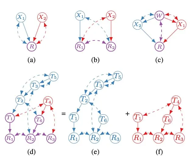
Figure showing examples of hedges, c-components, c-forests, and thickets. These form graphical criteria for g-identifiability. Details are discussed in the text itself. Thickets are shown to preclude g-identifiability. Crucially, (d) is shown to be an overlap of hedges which forms a thicket. Figure extracted from ³Lee, S., Correa, J. D., & Bareinboim, E. (2019). General identifiability with arbitrary surrogate experiments. UAI..

g-Identifiability ³Lee, S., Correa, J. D., & Bareinboim, E. (2019). General identifiability with arbitrary surrogate experiments. UAI.: Let $\boldsymbol{X}, \boldsymbol{Y}$ be disjoint sets of variables, $\mathbb{Z} = \{\boldsymbol{Z}_i\}_{i=1}^m$ be a collection of sets of variables, and let $\mathcal{G}$ be a causal diagram. If $P_x(y)$ is uniquely computable from distributions $\{ P(\boldsymbol{V} \mid do(z)) \}_{\boldsymbol{Z}\in\mathbb{Z}, \boldsymbol{z} \in dom(\boldsymbol{Z})}$ in any causal model which induces $\mathcal{G}$, we say that $P_x(y)$ is $g$-identifiable from $\mathbb{Z}$ in $\mathcal{G}$. Here $P(\boldsymbol{V})$ is the probability distribution describing the natural state of the system (assumed to be available).

Simply put, we say the distribution is $g$-identifiable with respect to a set of intervenable variables in the causal system if they are sufficient to uniquely compute it. This set of variables are the ones we intervene on by doing an experiment, as we discussed earlier. In this way it is a generalisation of $z$-identifiability discussed earlier. We now introduce some more definitions needed for the non-gID criteria.

Hedgelet decomposition ³Lee, S., Correa, J. D., & Bareinboim, E. (2019). General identifiability with arbitrary surrogate experiments. UAI.: The hedgelet decomposition of a hedge $\langle \mathcal{F}, \mathcal{F}^\prime \rangle$ is the collection of hedgelets $\{ \mathcal{F}(\boldsymbol{W}) \}_{\boldsymbol{W} \in \mathcal{C}(\mathcal{F}^{\prime\prime})}$ ($\mathcal{F}^{\prime\prime} = \mathcal{F}\setminus\mathcal{F}^{\prime}$) where each hedgelet $\mathcal{F}(\boldsymbol{W})$ is a subgraph of $\mathcal{F}$ made of (i) $\mathcal{F}[\boldsymbol{W}(\mathcal{F}) \cup \boldsymbol{W}]$ and (ii) $\mathcal{F}[De(\boldsymbol{W}_\mathcal{F})]$ without bidirected edges.

Referring back to the reference figure, some possible hedgelet decompositions are colour coded in blue and red to indicate distinct hedgelets, with purple used to indicate the shared variables (commonly root sets). This leads us nicely to the last definition we need for this criterion. Though this definition appears arbitrarily technical, it is rather intuitive once the reasoning is developed.

Thicket ³Lee, S., Correa, J. D., & Bareinboim, E. (2019). General identifiability with arbitrary surrogate experiments. UAI.: Let $\boldsymbol{R}$ be non-empty set of variables and $\mathbb{Z}$ be a collection of sets of variables in $\mathcal{G}$. A thicket $\mathcal{J} \subseteq \mathcal{G}$ is an $\boldsymbol{R}$-rooted c-component consisting of a minimal c-component over $\boldsymbol{R}$ and hedges $\mathbb{F}_{\mathcal{J}} = \{ \langle \mathcal{F}_{\boldsymbol{Z}}, \mathcal{J}[\boldsymbol{R}] \rangle \mid \mathcal{F}_{\boldsymbol{Z}} \subseteq \mathcal{G} \setminus \boldsymbol{Z}, \boldsymbol{Z} \cap \boldsymbol{R} = \emptyset \}_{\boldsymbol{Z} \in \mathbb{Z}}.$

Let’s consider this definition step-by-step by considering figure (c). First, we notice the graph is a c-component that contains a minimal c-component. It does not necessarily need to be a c-forest itself. Next, we need a pair of $\boldsymbol{R}$-rooted c-forests $\langle \mathcal{F}_{\boldsymbol{Z}}, \mathcal{J}[\boldsymbol{R}] \rangle$. We select the graphs induced by sets $\{W,X_1,R\}$ and $\{W,X_2,R\}$ with $\boldsymbol{Z} = \{\{X_1\},\{X_2\}\}$ the intervention set. Then we have hedges $\langle \mathcal{F}_{X_1}, \mathcal{J}[R] \rangle$ and $\langle \mathcal{F}_{X_2}, \mathcal{J}[R] \rangle$ that overlap and have intervention variables $Z\in\boldsymbol{Z}$ that do not intersect with the root set, $\boldsymbol{R}=\{R\}$. Basically, a thicket is an overlapping of hedges, and hedges were the ‘bad’ structure that prevented gID in the causal graph. Though this is a fairly involved procedure to do manually, especially on large causal graphs, it is algorithmically feasible as shown in Lee et al. The usefulness of this algorithm relies on the following result.

Thicket non-gID ³Lee, S., Correa, J. D., & Bareinboim, E. (2019). General identifiability with arbitrary surrogate experiments. UAI.: If there exists some thicket $\mathcal{J}$ for $P_{\boldsymbol{x}}(\boldsymbol{y})$ in causal graph $G$ with respect to intervention set $\mathbb{Z}$, then $P_{\boldsymbol{x}}(\boldsymbol{y})$ is not g-identifiable in $G$.

To make this idea explicit we include the following figure extracted from slides provided directly by Sanghack Lee, coauthor of several papers (including ³Lee, S., Correa, J. D., & Bareinboim, E. (2019). General identifiability with arbitrary surrogate experiments. UAI.) presented in this work ⁵Lee, S. (2020). General identifiability with arbitrary surrogate experiments. AAAI 2020 (presented at UAI 2019)..

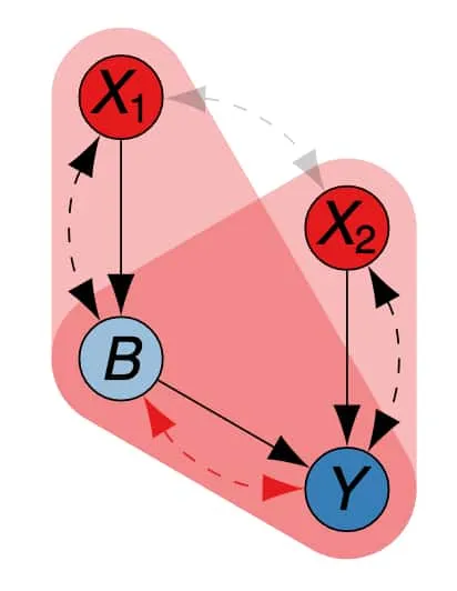
Thicket structure for $P_x(y)$ identified as an overlap of distinct hedges, each colours as a red rounded triangle. Extracted from ⁵Lee, S. (2020). General identifiability with arbitrary surrogate experiments. AAAI 2020 (presented at UAI 2019)..

This completes the required formalism’s for identifying structural constraints from explicit causal models. This ties well into the next section in which we discuss how we can apply this theory to learn causal structure from observational and interventional data. This is especially useful for allowing reinforcement learning agents to uncover causal structure.

Image credit: Header Image.

References

1. Bareinboim, E., & Pearl, J. (2014). Transportability from multiple environments with limited experiments: Completeness results. NIPS.
2. Bareinboim, E., & Pearl, J. (2016). Causal inference and the data-fusion problem. Proceedings of the National Academy of Sciences 113:7345–7352.
3. Lee, S., Correa, J. D., & Bareinboim, E. (2019). General identifiability with arbitrary surrogate experiments. UAI.
4. Tian, J., & Pearl, J. (2002). Studies in causal reasoning and learning.
5. Lee, S. (2020). General identifiability with arbitrary surrogate experiments. AAAI 2020 (presented at UAI 2019).

Comments are being migrated. Check back soon.