In the previous blog post we discussed some theory of how to select optimal and possibly optimal interventions in a causal framework. For those interested in the decision science, this blog post may be more inspiring. This next task involves applying counterfactual quantities to boost learning performance. This is clearly very important for an RL agent where its entire learning mechanism is based on interventions in a system. What if intervention isn’t possible? Let’s begin!

Counterfactual Decision Making

A key feature of causal inference is its ability to deal with counterfactual queries. Reinforcement learning, by its nature, deals with interventional quantities in a trial-and-error style of learning. Perhaps the most obvious question is: how can we implement RL in such a way as to deal with counterfactual and other causal factors in uncertain environments? In the preliminaries section we discussed the notions of a multi-armed bandit and their associated policy regret. This is a natural starting point for the merger of reinforcement learning and causal inference theory to solving counterfactual decision problems. We now discuss some interesting work done in this area, especially in the context of unobserved confounders in decision frameworks.

Obviously, the goal of optimising a policy is to minimise the regret an agent experiences. In addition, it should achieve this minimum regret as soon as possible in the learning process. Auer et al. ¹Auer, P., Cesa-Bianchi, N., & Fischer, P. (2004). Finite-time analysis of the multiarmed bandit problem. Machine Learning 47:235–256. show that policies can achieve logarithmic regret uniformly over time. Applying a policy they call UCB2, the authors show that with input $0 < \alpha < 1$ run on $K$ bandits (think slot machines), the expected regret after any number $n > \max_{i:\mu_i < \mu^\ast} \frac{1}{2 \Delta_i^2}$ of plays is bounded by

$\sum_{i:\mu_i < \mu^\ast} \left( \frac{(1+\alpha)(1+4\alpha\ln(2e\Delta_i^2 n))}{2\Delta_i} + \frac{c_\alpha}{\Delta_i} \right),$

where $\Delta_i = \mu_i^\ast - \mu_i$. Under different assumptions similar bounds can be achieved. Bareinboim et al. ²Bareinboim, E., Forney, A., & Pearl, J. (2015). Bandits with unobserved confounders: A causal approach. NIPS. show that these strategies are complicated by unobserved confounders when they are present in the data generating process. In fact, previous bandit algorithms implicitly attempt to maximise rewards by estimating experimental distributions. In other words, they attempt to optimise the procedure by calculating how their actions influence outcomes. This strategy fails to guarantee an optimal strategy in the wake of confounders - that is, unobserved factors in the system. Rephrasing the multi-armed bandit problem to account for unobserved confounders in causal language leads to a principle which exploits both observational and experimental modes of data to optimise reward. We now discuss this formalism in some detail with a motivating example in mind.

The following example is adapted from ²Bareinboim, E., Forney, A., & Pearl, J. (2015). Bandits with unobserved confounders: A causal approach. NIPS.. Imagine a casino with slot machines designed to detect whether a gambler is drunk. These machines are designed in such a way that they can attract drunk gamblers by flashing a light (stimulating some interest in drunk gamblers), knowing full well that drunk gamblers are less likely to notice machines tailoring payouts such that they are exploited. With full knowledge of gambling law, the casino devises a strategy to fool random testing strategies such that it appears the casino is following the legally required $30\%$ minimum payout. As enlightened scholars aware of causal inference theory, we have knowledge of the causal structure of the payout scheme and decide to condition on the intent of the gamblers. That is, we stratify data according to which machine a gambler intends to play, realising payout and intent are confounded by sobriety. The idea of an actor’s intent can be formalised. This will be very useful throughout CRL theory development.

Intent ³Forney, A., & Bareinboim, E. (2019). Counterfactual randomization: Rescuing experimental studies from obscured confounding. AAAI.: For all variables requiring an actor’s decision $\Pi_i \in \Pi$ in an SCM $M$, let the actor’s intended choice $I_{\Pi_i, t} = i_{\Pi_i, t}$ be the choice that the actor would make observationally for unit $t$ and the present unit’s configuration of UCs $U_t = u_t$. Formally, for parents of $\Pi_i$, $pa(\Pi_i)$, let $I_{\Pi_i, t} = f_{\Pi_i}(pa(\Pi_i)_t, u_{\Pi_i, t}).$

Applying the idea of conditioning on intent reveals gamblers are actually being paid $15\%$ (see tables below).

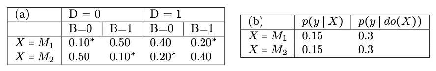
Table (a) encodes slot machine payout probabilities as found in the casino as a function of sobriety $D$, whether or not the machine has a flashing light $B$, and the machine type $X$. The ‘natural’ choices - or intent - of the gamblers are indicated by asterisks. Table (b) shows the observational and interventional probabilities of payouts when naively intervening on machines. Naive randomisation in the face of unobserved confounders (blinking light) fails to reveal the violation of gambling law. Tables recreated from ²Bareinboim, E., Forney, A., & Pearl, J. (2015). Bandits with unobserved confounders: A causal approach. NIPS..

K-Armed Bandit with Unobserved Confounders ²Bareinboim, E., Forney, A., & Pearl, J. (2015). Bandits with unobserved confounders: A causal approach. NIPS.: A K-Armed bandit problem with unobserved confounders is a causal model $M$ with reward distribution over $P(u)$ where:

1. $X_t \in \{ x_1,\dots,x_n \}$ is an observable encoding an agent’s arm choice from one of $k$ arms. This is decided naturally in the observational case, and by the policy in the experimental case, $do(X_t = \pi(x_0,y_0,\dots,x_{t-1},y_{t-1}))$ for strategy $\pi$.
2. $U_t$ represents the unobserved variable which affects the payout rate of arm $x_t$ by nature of influencing the agent’s choice.
3. $Y_t \in \{ 0,1 \}$ is a reward ($0$ indicates loss, $1$ indicates a win) for choosing arm $x_t$. This reward is determined by $y_t = f_y(x_t,u_t)$.

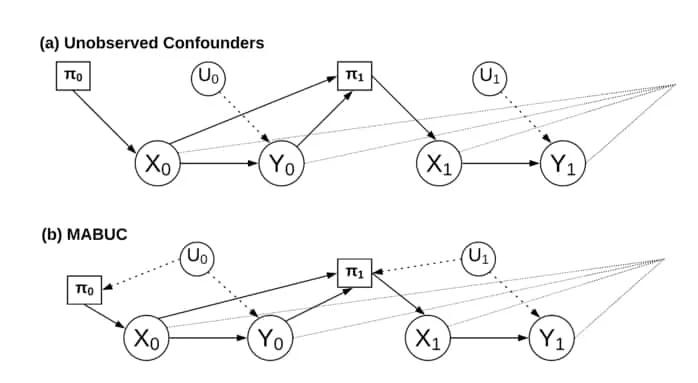
Diagram showing how unobserved confounder affects the MAB decision making process. (a) shows the standard MAB procedure in which only previous states and outcomes influence the policy. (b) shows the MABUC case in which unobserved confounders directly affect the policy of the agent. This changes how and what an agent can learn and is what ²Bareinboim, E., Forney, A., & Pearl, J. (2015). Bandits with unobserved confounders: A causal approach. NIPS. addresses. Figure created for this paper.

Allowing gamblers free roam of the casino floor to play slot machines as desired corresponds to the natural policy, $\pi_t$. This policy induces the observational distribution $P(y \mid x)$. Randomisation, on the other hand, removes external policies and corresponds to the interventional distribution $P(y \mid do(x))$. A major contribution of ²Bareinboim, E., Forney, A., & Pearl, J. (2015). Bandits with unobserved confounders: A causal approach. NIPS. is the extraction of information contained in both data-collection (observational and interventional) modes to understand and account for the players’ natural instincts. To perform such an analysis we need to consider counterfactuals: “would the agent win had it played on machine $M_i$ instead of $M_j$?” In other words, instead of considering $\textbf{argmax}_a \mathbb{E}[Y \mid do(X = a)]$ we should should be considering $\textbf{argmax}_a \mathbb{E}\left[ Y_{X=a} =1 \mid X = x \right],$ where $x$ represents the players intent and $a$ represents their final decision. This forms the regret decision criterion (RDC) - maximise the expected reward condition on the agents intent - and allows the following heuristic:

$\mathbb{E}(Y_{X=0} = 1 \mid X = 1) > \mathbb{E}(Y_{X=1} = 1 \mid X = 1)$

$\Leftrightarrow \mathbb{E}(Y_{X=0} = 1 \mid X = 1) > P(Y \mid X = 1).$

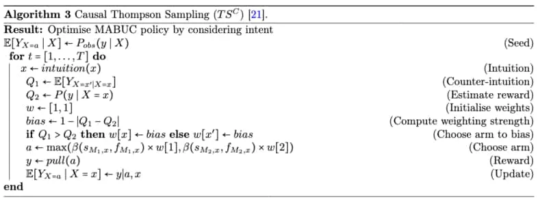
All this says is that we should consider the intent of the agent and consider how the causal system is trying to exploit this intent. The agent should acknowledge it’s own intent and modify its policy accordingly. The authors propose incorporating this into Thompson Sampling ⁴Thompson, W. R. (1933). On the likelihood that one unknown probability exceeds another in view of the evidence of two samples. Biometrika 25:285–294. to form Causal Thompson Sampling ($TS^C$), shown in the algorithm below. This algorithm leverages observational data to seed the algorithm and adds a rule to improve the arm exploration in the MABUC case. The algorithm is shown to dramatically improve convergence and regret against traditional methods under certain scenarios. Comments have been added to make the algorithm self-contained. The reader is encouraged to work through it.

The $TS^C$ is empirically shown to outperform conventional methods by converging upon an optimal policy faster and with less regret than the non-causally empowered approach. Ultimately we are interested in sequential decision making in the context of planning - the cases reinforcement learning addresses. ⁵Zhang, J., & Bareinboim, E. (2016). Markov decision processes with unobserved confounders: A causal approach. generalises the previous work on MABs to take a causal approach to Markov decision processes (MDPs) with unobserved confounders. In a similar fashion to ²Bareinboim, E., Forney, A., & Pearl, J. (2015). Bandits with unobserved confounders: A causal approach. NIPS., the authors construct a motivating example and show that MDP algorithms perform sub-optimally when applying conventional (non-causal) methods. First, we note why confounding in MDPs is different to confounding in MABs. Confounding in MDPs affects state and outcome variables in addition to action and outcome, and thus requires special treatment. Unlike in MABs, the MDP setting requires maximisation of reward over a long-term horizon (planning). Maximising with respect to the immediate future (greedy behaviour) thus fails to account for potentially superior long term trajectories in state-action space (long term strategies). The authors proceed by showing conventional MDP algorithms are not guaranteed to learn an optimal policy in the presence of unobserved confounders. Reformulating MDPs in terms of causal inference, we can show that counterfactual-aware policies outperform purely experimental algorithms.

MDP with Unobserved Confounders (MDPUC) ⁵Zhang, J., & Bareinboim, E. (2016). Markov decision processes with unobserved confounders: A causal approach.: A Markov Decision Process with Unobserved Confounders is an SCM $M$ with actions $X$, states $S$, and a binary reward $Y$:

1. $\gamma \in [0,1)$ is the discount factor.
2. $U^{(t)} \in U$ is the unobserved confounder at time-step $t$.
3. $V^{(t)} = X^{(t)} \cup Y^{(t)} \cup S^{(t)}$ is the set of observed variables at time-step $t$, where $X^{(t)} \in X$, $Y^{(t)} \in Y$, and $S^{(t)} \in S$.
4. $F = \{ f_x, f_y, f_s \}$ are the set o f structural equations relative to $V$ such that $X^{t} \leftarrow f_x(s^{(t)}, u^{(t)})$, $Y^{(t)} \leftarrow f_y(x^{(t)}, s^{(t)}, u^{(t)})$, and $S^{(t)} \leftarrow f_s(x^{(t-1)}, s^{(t-1)}, u^{(t-1)})$. In other words, they determine the next state and associated reward.
5. $P(u)$ encodes the probability distribution over the unobserved (exogenous) variables $U$.

A key difference to the MABUC case is that different sets of variables can be confounded over the time horizon. The following figure shows the four different ways in which MDPUC variables can be confounded.

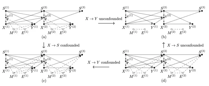
The figure above shows (a) MDPUC with action (decided by the policy) to reward path, $x^{(t)} \rightarrow y^{(t)}$ confounded. (b) MDP without confounders. This is the traditional RL instance. (c) MDPUC with action to reward path, $x^{(t)} \rightarrow y^{(t)}$, and action to state path, $x^{(t)} \rightarrow s^{(t+1)}$, confounded. (d) MDPUC with only action to state path, $x^{(t)} \rightarrow s^{(t+1)}$, confounded. Extracted from ⁵Zhang, J., & Bareinboim, E. (2016). Markov decision processes with unobserved confounders: A causal approach..

Most literature discussing reinforcement learning will develop the theory in terms of value functions. We develop these notions for the MDPUC case here. This will allow us (in theory) to exploit existing RL literature with relative ease.

Value Functions: Given a MDPUC model $M\langle \gamma, U, X, Y, S, F, P(u) \rangle$ and an arbitrary deterministic policy $\pi$, we can define the value function starting from state $s^{(t)}$, taking action $x^{(t)}$, and thereafter following policy $\pi$ as: $V^{\pi}(s^{(t)}) = \mathbb{E}\left[ \sum_{k=0}^{\infty} \gamma^k Y_{x^{([t, t+k])} = \pi}^{(t+k)} \mid s^{(t)} \right].$ The state-action value function is similarly defined: $Q^{\pi}(s^{(t)}, x^{(t)}) = \mathbb{E}\left[ \sum_{k=0}^{\infty} \gamma^k Y_{x^{(k)}, x^{([t+1, t+k])} = \pi}^{(t+k)} \mid s^{(t)}, x^{(t)} \right].$

The interpretation of these functions is the same as in the usual RL literature. They simply associate a state or state-action with an expected reward over all future time steps. Using these definitions, we can derive expressions for the well known Bellman equation and recursive definitions for the state and state-action value functions ⁶Sutton, R. S., & Barto, A. G. (2018). Reinforcement Learning: An Introduction. MIT Press (2nd ed.). for the situation where unobserved confounders are present. The authors rest their analysis of these results on the axioms of counterfactuals and the Markov property presented in theorem (\ref{thm

}). Proofs for the following theorems are available in the source paper ⁵Zhang, J., & Bareinboim, E. (2016). Markov decision processes with unobserved confounders: A causal approach. and are not included here for brevity.

Markovian Property in MDPUCs ⁵Zhang, J., & Bareinboim, E. (2016). Markov decision processes with unobserved confounders: A causal approach.: For a MDPUC model M $\langle \gamma, U, X, Y, S, F, P(u) \rangle$, a policy $\pi \in F_{exp} = \{ \pi \mid \pi: S \rightarrow X \}$ (state to action map), and a starting state $s^{(t)}$, the agents performs actions $do(X^{(t)} = x^{(t)})$ at round $t$ and $do(X^{([t+1,t+k])} = \pi)$ afterwards $(k \in \mathbb{Z}^+)$, the following statement holds:

$P\left(Y_{x^{(t)}, x^{([t+1, t+k])}=\pi}^{t+k}=y^{(t+k)} \mid s_{x^{(t)}}^{(t+1)}, s^{(t)}\right)=P\left(Y_{x^{([t+1, t+k])}=\pi}^{t+k}=y^{(t+k)} \mid s^{(t+1)}\right)$

We can further extend MDPUCs to counterfactual policies by considering $F_{ctf} = \{ \pi \mid \pi: S \times X \rightarrow X \}$, the set of functions between the current state $s^{(t)}$, the intuition of the agent $x^{\prime(t)}$, and the action $x^{(t)}$. Then $V^{(t)} = V^{(t)}(s^{(t)},x^{\prime(t)})$ and $Q^{(t)} = Q^{(t)}(s^{(t)}, x^{\prime(t)}, x^{(t)})$. With this we can derive a remarkable result encoded as a theorem below.

Theorem: Given an MDPUC instance $M\langle \gamma, U, X, Y, S, F, P(u) \rangle$, let $\pi_{exp}^\ast = \textbf{argmax}_{\pi \in F_{exp}} V^{\pi}(s^{(t)})$ and $\pi_{ctf}^\ast = \textbf{argmax}_{\pi \in F_{ctf}} V^{\pi}(s^{(t)}, x^{\prime(t)})$. For any state $s^{(t)}$, the following statement holds: $V^{\pi_{exp}^\ast}(s^{(t)}) \leq V^{\pi_{ctf}^\ast}(s^{(t)}).$ In other words, we can never do worse by considering counterfactual quantities (intent).

Zhang and Bareinboim ⁵Zhang, J., & Bareinboim, E. (2016). Markov decision processes with unobserved confounders: A causal approach. continue to implement a counterfactual-aware MORMAX MDP algorithm and empirically show it superior to conventional MORMAX ⁷Szita, I., & Szepesvári, C. (2010). Model-based reinforcement learning with nearly tight exploration complexity bounds. ICML. approaches in intent-sensitive scenarios. Forney and Bareinboim ⁸Bareinboim, E., & Pearl, J. (2016). Causal inference and the data-fusion problem. Proceedings of the National Academy of Sciences 113:7345–7352. extend this counterfactual awareness to the design of experiments.

Forney, Pearl and Bareinboim ⁹Forney, A., Pearl, J., & Bareinboim, E. (2017). Counterfactual data-fusion for online reinforcement learners. ICML. expand upon the ideas presented above by showing that counterfactual-based decision-making circumvents problems of naive randomisation when UCs are present. The formalism presented coherently fuses observational and experimental data to make well informed decisions by estimating counterfactual quantities empirically. More concretely, they study conditions under which data collected from distinct sources and conditions can be combined to improve learning performance by an RL agent. The key insight here is that seeing does not equate to doing in the world of data. Applying a developed heuristic, a variant of Thompson Sampling ⁴Thompson, W. R. (1933). On the likelihood that one unknown probability exceeds another in view of the evidence of two samples. Biometrika 25:285–294. is introduced and empirically shown to outperform previous state-of-the-art agents. An extension of the motivating example of (potentially) drunk gamblers from ²Bareinboim, E., Forney, A., & Pearl, J. (2015). Bandits with unobserved confounders: A causal approach. NIPS. is extended to consider an extra dependence on whether or not all the machines have blinking lights. This yields four combinations of the states of sobriety and blinking machines.

We start by noticing the interventional quantities, $\mathbb{E}[Y \mid do(X=x)]$ can be written in terms of counterfactuals as $\mathbb{E}[Y_{X=x}] = \mathbb{E}[Y_x]$ - that is, the expected value of $Y$ had $X$ been $x$. Applying the law of total probabilities, we arrive at the useful representation

$\mathbb{E}[Y_x] = \mathbb{E}[Y_x \mid x_1]P(x_1) + \dots + \mathbb{E}[Y_x \mid x_K]P(x_K).$

$\mathbb{E}[Y_x]$ is interventional by definition. $\mathbb{E}[Y_x \mid x^\prime]$ is either observational or counterfactual depending on whether $x=x^\prime$ or $x \neq x^\prime$ respectively. That is, whether or not $x^\prime$ has occurred. As we noted earlier, counterfactual quantities are, by their nature, not empirically available in general. Interestingly, however, intents of the agent contain information about the agent’s decision process and can reveal encoded information about unobserved confounders, as we noted in the MAB case earlier. Applying randomisation to intent conditions (with RDC) can allow computation of counterfactual quantities. In this way, observational data actually adds information to the seemingly more informative interventional data. This counterfactual quantity - that is not naturally realisable - is often referred to as the effect of the treatment on the treated ¹⁰Heckman, J. (1991). Randomization and social policy evaluation., by way of the fact that doctors cannot retroactively observe how changing the treatment would have affected a specific patient - well, they shouldn’t!

Estimation of ETT ⁹Forney, A., Pearl, J., & Bareinboim, E. (2017). Counterfactual data-fusion for online reinforcement learners. ICML.: The counterfactual quantity referred to as the effect of the treatment on the treated (ETT) is empirically estimable for any number of action choices when agents condition on their intent $I=i$ and estimate the response $Y$ to their final action choice $X=a$.

Proof: The ETT counterfactual quantity can be written as $\mathbb{E}[Y_{X=a} \mid X = i]$. Applying law of total probability and conditional independence relation $Y_x \perp X \mid I$, we have:

$$\begin{aligned} \mathbb{E}\left[Y_{X=a} \mid X=i\right] &=\sum_{i^{\prime}} \mathbb{E}\left[Y_{X=a} \mid X=i, I=i^{\prime}\right] P\left(I=i^{\prime} \mid X=i\right) \\ &=\sum_{i^{\prime}} \mathbb{E}\left[Y_{X=a} \mid I=i^{\prime}\right] P\left(I=i^{\prime} \mid X=i\right) \end{aligned}$$

Now, we notice that $I_x = I$ because in $G_{\overline{X}}$ (graph with edges into $X$ removed) we have $(I \perp X)_{G_{\overline{X}}}$. Thus,

$$\begin{aligned} \mathbb{E}\left[Y_{X=a} \mid X=i\right] &=\sum_{i^{\prime}} \mathbb{E}\left[Y_{X=a} \mid I=i^{\prime}\right] P\left(I=i^{\prime} \mid X=i\right) \\ &=\sum_{i^{\prime}} \mathbb{E}\left[Y_{X=a} \mid I_{x=a}=i^{\prime}\right] P\left(I=i^{\prime} \mid X=i\right) \\ &=\sum_{i^{\prime}} \mathbb{E}\left[Y \mid d o(X=a), I=i^{\prime}\right] P\left(I=i^{\prime} \mid X=i\right) \end{aligned}$$

where the last line follows since all quantities are in relation to the same variable $x$ and so the counterfactual quantity can be written as an interventional quantity. We now notice that since $P(I = i^\prime \mid X = i)$ is observational, the intent will always match the outcome. We can thus rewrite this as an indicator function. The result follows.

$$\begin{aligned} \mathbb{E}\left[Y_{X=a} \mid X=i\right] &=\sum_{i^{\prime}} \mathbb{E}\left[Y \mid d o(X=a), I=i^{\prime}\right] P\left(I=i^{\prime} \mid X=i\right) \\ &=\sum_{i^{\prime}} \mathbb{E}\left[Y \mid d o(X=a), I=i^{\prime}\right] \mathbb{1}_{i^{\prime}=i} \\ &=\mathbb{E}[Y \mid d o(X=a), I=i] \end{aligned}$$

⁹Forney, A., Pearl, J., & Bareinboim, E. (2017). Counterfactual data-fusion for online reinforcement learners. ICML. makes use of this result to suggest heuristics for learning counterfactual quantities from (possibly noisy) experimental and observational data.

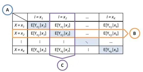
This figure shows the counterfactual possibilities for different actions and action-intents. The diagonal indicates the counterfactual quantities that have occurred. We can apply knowledge of other counterfactual quantities to learn about other possible counterfactuals. (B) indicates cross-intent learning. (C) indicates cross-arm learning. Extracted form ⁹Forney, A., Pearl, J., & Bareinboim, E. (2017). Counterfactual data-fusion for online reinforcement learners. ICML..

1. Cross-Intent Learning: Thinking about these equation carefully, we notice that since they holds for every arm, we have a system of equations for outcomes conditioned on different intents. Thus to find $\mathbb{E}[Y_{x_r} \mid x_w]$ we can learn about other intent conditions: $\mathbb{E}[Y_{x_r} \mid x_w] = \left[\mathbb{E}[Y_{x_r}] - \sum_{i \neq w}^K \mathbb{E}[Y_{x_r} \mid x_i] P(x_i)\right] / P(x_w).$

2. Cross-Arm Learning: Similarly to (1), we can observe that given information about two different arms under the same intent, we can learn about a third arm under the same intent. We have

   $P\left(x_w\right)=\frac{E\left[Y_{x_{r}}\right]-\sum_{i \neq w}^{K} E\left[Y_{x_{r}} \mid x_{i}\right] P\left(x_{i}\right)}{E\left[Y_{x_{r}} \mid x_{w}\right]}$

   Which is the same as writing

   $P\left(x_w\right)=\frac{E\left[Y_{x_{s}}\right]-\sum_{i \neq w}^{K} E\left[Y_{x_{s}} \mid x_{i}\right] P\left(x_{i}\right)}{E\left[Y_{x_{s}} \mid x_{w}\right]}$

   Combining these results and solving for $\mathbb{E}[Y_{x_r} \mid x_w]$ we find:

   \begin{equation} \label{eqn

   } E\left[Y_{x_{r}} \mid x_{w}\right]=\frac{\left[E\left[Y_{x_{r}}\right]-\sum_{i \neq w}^{K} E\left[Y_{x_{r}} \mid x_{i}\right] P\left(x_{i}\right)\right] E\left[Y_{x_{s}} \mid x_{w}\right]}{E\left[Y_{x_{s}}\right]-\sum_{i \neq w}^{K} E\left[Y_{x_{s}} \mid x_{i}\right] P\left(x_{i}\right)}. \end{equation}

   This estimate is not robust to noise in the samples. We can take a pooling approach and account for variance of reward payouts by applying an inverse-variance-weighted average: $E_{X A r m}\left[Y_{x_{r}} \mid x_{w}\right]=\frac{\sum_{i \neq r}^{K} h_{XArm}\left(x_{r}, x_{w}, x_{i}\right) / \sigma_{x_{i}, x_{w}}^{2}}{\sum_{i \neq r}^{K} 1 / \sigma_{x_{i}, x_{w}}^{2}},$ where $h_{XArm}\left(x_{r}, x_{w}, x_{s}\right)$ evaluates equation (\ref{eqn

   }), and $\sigma_{x_{i}, i}^2$ is the reward variance for arm $x$ under intent $i$.

3. Combined Approach: Of course, we can combine the previous two approaches by sampling (collecting) estimates during execution and applying cross-intent and cross-arm learning strategies. A fairly straightforward derivation yields a combined approach formula:

   $E_{\text {combo}}\left[Y_{x_{r}} \mid x_{w}\right]=\frac{\alpha}{\beta}, \quad \text{where}$

   $\alpha = E_{\text {samp}}\left[Y_{x_{r}} \mid x_{w}\right] / \sigma_{x_{r}, x_{w}}^{2}+E_{\text {XInt}}\left[Y_{x_{r}} \mid x_{w}\right] / \sigma_{X \text {Int}}^{2} +E_{\text {XArm}}\left[Y_{x_{r}} \mid x_{w}\right] / \sigma_{X A r m}^{2}$

   $\beta = 1 / \sigma_{x_{r}, x_{w}}^{2}+1 / \sigma_{X \text {Int}}^{2}+1 / \sigma_{X A r m}^{2}$

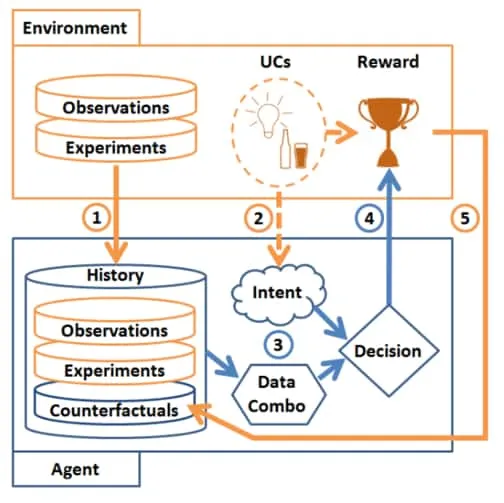
This figure shows the flow and process of fusing data using counterfactual reasoning as outlined in this section. The agent employs both the history of interventional and observational data to compute counterfactual quantities. Along with its intended action, the agent makes a counterfactual and intent aware decision to account for unobserved confounders and make use of available information. Figure extracted from ⁹Forney, A., Pearl, J., & Bareinboim, E. (2017). Counterfactual data-fusion for online reinforcement learners. ICML..

The authors proceed to experimentally verify that this data-fusion approach, applied to Thompson Sampling, results in significantly less regret than competitive MABUC algorithms. The (conventional) gold standard for dealing with unobserved confounders involves randomised control trials (RCTs) ¹¹Fisher, R. A. (1935). The Design of Experiments. Oliver and Boyd., especially useful in medical drug testing, for example. As we noted in the data-fusion and earlier MABUC processes, randomisation of treatments may yield population-level treatment outcomes but can fail to account for individual-level characteristics. The authors provide a motivating example in the domain of personalised medicine, or the effect of the treatment on the treated, motivated by Stead et al.’s ¹²Stead, W. W., Starmer, J. M., & McClellan, M. (2008). Beyond expert based practice. Evidence-Based Medicine and the Changing Nature of Healthcare (IOM). observation that

Despite their attention to evidence, studies repeatedly show marked variability in what healthcare providers actually do in a given situation. - Stead et al.’s ¹²Stead, W. W., Starmer, J. M., & McClellan, M. (2008). Beyond expert based practice. Evidence-Based Medicine and the Changing Nature of Healthcare (IOM).

They proceed to formalise the existence of different treatment policies of actors in confounded decision-making scenarios. This new theory is applied to generalise RCT procedures to allow recovery of individualised treatment effects from existing RCT results. Further, they present an online algorithm which can recommend actions in the face of multiple treatment opinions in the context of unobserved confounders. For the sake of clarity, the motivating example is now briefly presented. The reader is encouraged to refer to the source material ³Forney, A., & Bareinboim, E. (2019). Counterfactual randomization: Rescuing experimental studies from obscured confounding. AAAI. for further details.

Consider two drugs which appear to be equally effective under an FDA-approved RCT. In practice, however, one physician finds agreement with the RCT results while another does not. Let us consider two potential unobserved confounders - socioeconomic status (SES) and the patient’s treatment request (R). Crucially, we note that juxtaposing observational and experimental data fails to reveal these invisible confounders. Key to this confounded decision making (CDM) scenario is that the deciding agent (physician) do not possess a fully specified causal model (in the form of an SCM). This formalism was used to define a regret decision criterion (RDC) for optimising actions in the face of unobserved confounders. In the physician motivating example we just discussed, the intent-specific recovery rates of the first physician do not appear to differ from the observational or interventional recovery rates. The results of RDC for the second physician is only slightly off the data, at $72.5\%$. What is happening here? The key here is the heterogeneous intents of the agents. We now develop theory to account and exploit information implicitly contained in the multiple intents of agents.

Heterogeneous Intents ³Forney, A., & Bareinboim, E. (2019). Counterfactual randomization: Rescuing experimental studies from obscured confounding. AAAI.: Let $A_1$ and $A_2$ be two actors within a CDM instance, and $M^{A_1}$ be the SCM associated with the choice of policies of $A_1$ and likewise $M^{A_2}$ of $A_2$. For any decision variable $X \in \Pi_M$ and its associated intent $I = f_x$, the actors are said to have heterogeneous intent in $f_I^{A_1} \in F_M^{A_1}$ and $f_I^{A_2} \in F_M^{A_2}$ are distinct.

Acknowledging the possibility of heterogeneous intents in deciding actors (such as second opinions), we can extend the notion of SCMs. The figure below shows a model for combining intents of different agents.

HI Structural Causal Model (HI-SCM) ³Forney, A., & Bareinboim, E. (2019). Counterfactual randomization: Rescuing experimental studies from obscured confounding. AAAI.: A heterogeneous intent structural causal model $M^{\boldsymbol{A}}$ is an SCM that combines the individual SCMs of actors $\boldsymbol{A} = \{ A_{1}, \dots, A_{a} \}$ such that each decision variable in $M^{\boldsymbol{A}}$ is a function of each actors’ individual intents.

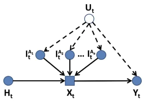
This figure shows an example of HI-SCM. Here multiple intents of different actors contribute to the decision variable $X_t$. Unobserved confounder $U_t$ affects both the intents and the outcome. The agent history is encoded as $H_t$. Recreated based on figure 1 in ³Forney, A., & Bareinboim, E. (2019). Counterfactual randomization: Rescuing experimental studies from obscured confounding. AAAI..

Of course, it would be naive to assume every actor adds valuable information to the total knowledge of the system. With this is mind, we develop the notion of an intent equivalence class.

Intent Equivalence Class (IEC) ³Forney, A., & Bareinboim, E. (2019). Counterfactual randomization: Rescuing experimental studies from obscured confounding. AAAI.: In a HI-SCM $M^A$, we say that any two actors $A_i \neq A_j$ belong to separate intent equivalence classes $\boldsymbol{\Phi} = \{ \phi_1, \dots, \phi_m \}$ of intent functions $f_I$ if $f_I^{A_i} \neq f_I^{A_j}$.

With this definition in place, we can cluster equivalent actors - and their associated intents - by their IEC. For example, given $\phi_1 = \{ A_1, A_2 \}$ then

$P(Y_x \mid I^{A_1}) = P(Y_x \mid I^{A_2}) = P(Y_x \mid I^{A_1}, I^{A_2}) = P(Y_x \mid I^{\phi_1}).$

It turns out that IEC-specific optimisation is always at least equivalent to each actor’s individual optimal action.

IEC-Specific Reward Superiority ³Forney, A., & Bareinboim, E. (2019). Counterfactual randomization: Rescuing experimental studies from obscured confounding. AAAI.: Let $X$ be a decision variable in a HI-SCM $M^A$ with measured outcome $Y$, and let $I^{\phi_i}$ and $I^{\phi_j}$ be the heterogeneous intents of two distinct IECs $\phi_i, \phi_j$ in the set of all IECs in the system, $\boldsymbol{\Phi}$. Then

$\max_{x \in X} P(Y_x \mid I^{\phi_i}) \leq \max_{x \in X} P(Y_x \mid I^{\phi_i}, I^{\phi_j}) \quad \forall \phi_i, \phi_j \in \boldsymbol{\Phi}.$

Proof: WLOG, consider the case of a binary intents $X$. Let $x^* = \textbf{argmax}_{x \in X} P(Y_x \mid I^{\phi_i} = i^{\phi_i}).$ Then

$P\left(Y_{x}^{*} \mid I^{\phi_{i}}=i^{\phi_{i}}\right)>P\left(Y_{x}^{\prime} \mid I^{\phi_{i}}=i^{\phi_{i}}\right)$

$\Longrightarrow \sum_{i^{\phi_{j}}} P\left(Y_{x^{*}} \mid I^{\phi_{i}}=i^{\phi_{i}}, I^{\phi_{j}}=i^{\phi_{j}}\right) P\left(I^{\phi_{j}}=i^{\phi_{j}} \mid I^{\phi_{i}}=i^{\phi_{i}}\right)$

$>\sum_{i^{\phi_{j}}} P\left(Y_{x^{\prime}} \mid I^{\phi_{i}}=i^{\phi_{i}}, I^{\phi_{j}}=i^{\phi_{j}}\right) P\left(I^{\phi_{j}}=i^{\phi_{j}} \mid I^{\phi_{i}}=i^{\phi_{i}}\right)$

Letting $p = P\left(I^{\phi_{j}}=i^{\phi_{j}} \mid I^{\phi_{i}}=i^{\phi_{i}}\right),$ we can rewrite the above inequality as $a(p) + b(1-p) > c(p) + d(1-p)$ (corrected mistake from proof in appendix of source). We can write it as such since we are considering the binary case. Thus if we have one case occurs, necessarily the other doesn’t. We can then exhaust the cases:

1. $p = 0 \implies b > d$.
2. $p = 1 \implies a > c$.
3. $p \in (0,1) \implies \max(a,b) \geq a(p) + b(1-p)$.

Thus, in each case we have that the HI-specific rewards are greater than or equal to the homogeneous-intent-specific rewards.

With this important result in place, we can develop new criteria for decision making in a CDM with heterogeneous intents.

HI Regret Decision Criteria (HI-RDC) ³Forney, A., & Bareinboim, E. (2019). Counterfactual randomization: Rescuing experimental studies from obscured confounding. AAAI.: In a CDM scenario modelled by a HI-SCM $M^A$ with treatment $X$, outcome $Y$, actor intended treatments $I^{A_i}$, and a set of actor IECs $\boldsymbol{\Phi} = \{ \phi_1, \dots, \phi_m \}$, the optimal treatment $x^\ast \in X$ maximises the IEC-specific treatment outcome. Formally: $x^\ast = \textbf{argmax}_{x \in X} P(Y_x \mid I^{\phi_1}, \dots, I^{\phi_m}).$

The authors point out that HI-RDC requires knowledge of IECs, which are not always obvious. This motivates the need for empirical means of clustering the actors into equivalence classes. Since these intents are observational (they are indicated by what naturally occurs), sampling and grouping by the following criteria suffices.

Empirical IEC Clustering Criteria ³Forney, A., & Bareinboim, E. (2019). Counterfactual randomization: Rescuing experimental studies from obscured confounding. AAAI.: Let $A_i$, $A_j$ be two agents modelled by a HI-SCM, and let their associated intents be $I^{A_i}$, $I^{A_j}$ for some decision. We cluster agents into the same IEC, $\{ A_i, A_j \} \in \phi_r$, whenever their intended actions over the same units correlate. In other words, if their intent-specific treatment outcomes will agree. Correlation indicated by $\rho$, as is common in statistics literature. Formally:

$$\begin{aligned} \rho\left(I^{A_{i}}, I^{A_{j}}\right)=1 & \Longrightarrow\left\{A_{i}, A_{j}\right\} \in \phi_{r} \in \Phi \\ & \Longrightarrow P\left(Y_{x} \mid I^{A_{i}}\right)=P\left(Y_{x} \mid I^{A_{i}}, I^{A_{j}}\right) \end{aligned}$$

The authors argue that this condition can be too strict in practice and should be softened to allow for some actor-specific noise. Applying HI-RDC and empirical IEC clustering directly to the online recommendation system presented in ²Bareinboim, E., Forney, A., & Pearl, J. (2015). Bandits with unobserved confounders: A causal approach. NIPS. is possible but not necessarily always practical or recommended because (1) the ethics of exploring different treatment options is not always clear and (2) if UCs are present in the system and the treatment has passed experimental testing, this implies that the UCs have gone unnoticed and we - the data analysts - wouldn’t necessarily know to look for them there. This motivates the need for an extension to RCTs to involve heterogeneous intents.

HI Randomised Control Trial (HI-RDC) ³Forney, A., & Bareinboim, E. (2019). Counterfactual randomization: Rescuing experimental studies from obscured confounding. AAAI.: Let $X$ be the treatment of the RCT in which all participants of the trial are randomly assigned to some experimental condition. In other words, they have been intervened on via $do(X=x)$ with some measured outcome $Y$. Let $\boldsymbol{\Phi}$ be the set of all IECs for agents in the HI-SCM $M^A$ for which the RCT is meant to apply. A Heterogeneous Intent RCT (HI-RCT) is an RCT wherein treatments are randomly assigned to each participant but, in addition, the intended treatments of the sampled agents are collected for each participant.

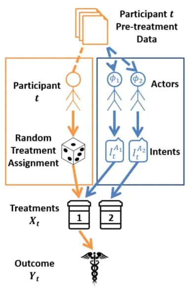
This figure shows the HI-RDC procedure. The traditional RCT procedure is found by following the orange path. HI-RDC adds an additional layer of actor-intent collection over and above the traditional RCT procedure. Figure extracted form ³Forney, A., & Bareinboim, E. (2019). Counterfactual randomization: Rescuing experimental studies from obscured confounding. AAAI..

This procedure yields actor IECs as well as experimental, observational, counterfactual and HI-specific treatment effects. Finally, we can implement a criterion which reveals confounding beyond what a simple mix of observational and interventional data can expose.

HI-RDC Confounding Criteria ³Forney, A., & Bareinboim, E. (2019). Counterfactual randomization: Rescuing experimental studies from obscured confounding. AAAI.: Consider a CDM scenario modelled by a HI-SCM $M^A$ with treatment $X$, outcome $Y$, actor intended treatments $I^{A_i}$, and a set of actor IECs $\Phi = \{ \phi_i, \dots, \phi_m \}$. Whenever there exists some $x \in X, i^{\Phi} \in I^{\Phi} : P(Y_x) \neq P(Y_x \mid i^{\Phi})$ in $M^A$, then there exists some unobserved $U$ such that $X \leftarrow U \rightarrow Y$.

In addition to the above theory, ³Forney, A., & Bareinboim, E. (2019). Counterfactual randomization: Rescuing experimental studies from obscured confounding. AAAI. provides a procedure for an agent to attempt to repair harmful influences of unobserved confounders in an online procedure. Once again we come across the Multi-Armed Bandit with Unobserved Confounders (MABUC) in the attempt to maximise the reward (recovery in the physician example) - or minimise the regret - of the decision making process. One problem that arises in the online case is that the IECs the agent learns are not necessarily exhausitive. Let us consider whether we can find a mapping $\Phi_{on} \rightarrow \Phi_{off}$, representing a map from the online to the offline IEC sets respectively. If we can, the HI-RDC reveals optimal treatment. If not, HI-RCT data can be used to accelerate learning by gathering a calibration unit set - a small sample questionnaire in which actors are asked to provide intended treatments. In the case where HI-RCT IECs correspond to the sampled offline IECs, a mapping can be made. This acts as a sort of ‘bootstrap’ to the HI-RCT procedure by serving as a procedure to collect initial conditions for the learning process.

Actor Calibration-Set Heuristic ³Forney, A., & Bareinboim, E. (2019). Counterfactual randomization: Rescuing experimental studies from obscured confounding. AAAI.: A collection of some $n > 0$ calibration units from an offline HI-RDC dataset $\mathcal{D}$ can be used to learn the IECs of agents in an online domain. Three heuristics scores $h(t) = h_c(t) + h_d(t) + h_o(t)$ can be used to guide the selection procedure:

1. Consistency: how consistent agents in the same IEC $\phi_r = \{ A_1, \dots, A_i \}$ are with their intended treatment,

   $h_c(t) = \text{Number of } I_t^A \in \phi_r \text{ agreeing with majority }/\mid\phi_{r}\mid$.

2. Diversity: how often a configuration of $I^\Phi$ has been chosen, favouring a diverse set of IEC intent combinations, $h_d(t) = 1/(\text{Number of times } I^\Phi \text{ appears in calibration set})$. This acts by favouring ‘exploration’ in terms of the IEC space.

3. Optimism: a bias towards choosing units in which the randomly assig ned treatment $x_t$ was optimal and succeeded or suboptimal and failed,

$h_o(t) = \left(P\left(Y_{x_{t}} \mid I_{t}^{\Phi}\right)>P\left(Y_{x^{\prime}} \mid I_{t}^{\Phi}\right) \forall x^{\prime} \in X \backslash x_{t}\right) 1\left(Y_{t}=1\right)$

$+\left(P\left(Y_{x_{t}} \mid I_{t}^{\Phi}\right)<P\left(Y_{x^{\prime}} \mid I_{t}^{\Phi}\right) \exists x^{\prime} \in X \backslash x_{t}\right) 1\left(Y_{t}=0\right)$

The calibration set is given by $h(\mathcal{D}, n) = \{ t \in \mathcal{D} \mid n \text{ highest } h(t) \}$.

The authors experimentally show that agents maximising HI-specific rewards, clustering by IEC, and using calibration sets with and without the Actor Calibration-Set Heuristic, each outperforms the previous version. In other words, each step improves upon the regret the agent experiences. When compared against an oracle - that treated UCs as observed (unrealisable) - the agent performs well. ¹³Zhang, J., & Bareinboim, E. (2020). Can humans be out of the loop?. asks some interesting questions and presents intriguing results. They tackle the problem of an agent and humans having different sensory capabilities, and thereby “disagreeing” on their observations. The authors find that when leaving human intuition out of the loop - even when the agent’s sensory abilities are superior - results in worse performance. The theory presented in this section is sufficient to understand the presentation of the results in ¹³Zhang, J., & Bareinboim, E. (2020). Can humans be out of the loop?., and the reader is encouraged to engage with the source.

Now that we have considered counterfactual decision making within a causal system, we should consider how we can transfer and generalise causal results across domains. This is what the next section tackles.

Image credit: Header Image.

References

1. Auer, P., Cesa-Bianchi, N., & Fischer, P. (2004). Finite-time analysis of the multiarmed bandit problem. Machine Learning 47:235–256.
2. Bareinboim, E., Forney, A., & Pearl, J. (2015). Bandits with unobserved confounders: A causal approach. NIPS.
3. Forney, A., & Bareinboim, E. (2019). Counterfactual randomization: Rescuing experimental studies from obscured confounding. AAAI.
4. Thompson, W. R. (1933). On the likelihood that one unknown probability exceeds another in view of the evidence of two samples. Biometrika 25:285–294.
5. Zhang, J., & Bareinboim, E. (2016). Markov decision processes with unobserved confounders: A causal approach.
6. Sutton, R. S., & Barto, A. G. (2018). Reinforcement Learning: An Introduction. MIT Press (2nd ed.).
7. Szita, I., & Szepesvári, C. (2010). Model-based reinforcement learning with nearly tight exploration complexity bounds. ICML.
8. Bareinboim, E., & Pearl, J. (2016). Causal inference and the data-fusion problem. Proceedings of the National Academy of Sciences 113:7345–7352.
9. Forney, A., Pearl, J., & Bareinboim, E. (2017). Counterfactual data-fusion for online reinforcement learners. ICML.
10. Heckman, J. (1991). Randomization and social policy evaluation.
11. Fisher, R. A. (1935). The Design of Experiments. Oliver and Boyd.
12. Stead, W. W., Starmer, J. M., & McClellan, M. (2008). Beyond expert based practice. Evidence-Based Medicine and the Changing Nature of Healthcare (IOM).
13. Zhang, J., & Bareinboim, E. (2020). Can humans be out of the loop?.

Comments are being migrated. Check back soon.