And as quickly as that, we’re at task 6 of our quest. Causal imitation learning is perhaps the most fanciful-sounding, but at it’s core it remains as simple a goal as the challenge presented by Abbeel and Ng in 2004. The really exciting part here is that we have rigorous methods for combining our causal techniques with imitation learning procedures using RL. This is a really cutting edge research area and we only discuss one paper in detail here. Keep an eye out for exciting developments coming from left, right and centre!

This Series

Causal Imitation Learning

We now reach the final task presented by Bareinboim in his development of the causal reinforcement learning framework [9]. This task involves the interesting challenge of learning by expert demonstration - imitation learning. In their now classic paper, Abbeel and Ng [48] explored applying inverse reinforcement learning (IRL) techniques to the imitation learning procedure. Essentially, IRL learns a reward function that emphasises the observed expert trajectories. This is in contrast to the other common method of imitation learning known as behaviour cloning where an agent seeks to mimic the policy of the expert. Both these methods have been successful in their own right, but they make the strong assumption that actions of the expert are fully observed by the imitator. [49] addresses some of these shortcomings by introducing a complete graphical criterion for determining whether imitation learning is feasible given observational data and knowledge about the underlying causal process. Further, a sufficient algorithm for identifying an imitation policy when this criterion does not hold is presented.

Partially Observable SCM [49]: A POSCM is a tuple $\langle M, \boldsymbol{O}, \boldsymbol{L} \rangle$. Here $M$ is an SCM, $\boldsymbol{O}$ represents the observed endogenous variables, and $\boldsymbol{L}$ represents the latent (unobserved) endogenous variables. The observed and latent variables are mutually exhaustive over the endogenous variables.

The task at hand is to determine the value of performing some intervention (action) that is part of the observed variable set, $X \in \boldsymbol{O}$. Assuming the reward is latent, we wish to identify a policy $\pi$ such that the expected reward $\mathbb{E}[Y \mid do(\pi)]$ exceeds a certain minimum performance requirement, $\tau$. We say $P(y \mid do(\pi))$ is identifiable if for a subset of the exogenous variables, $\boldsymbol{Y} \subseteq \boldsymbol{V}$, the distribution $P(y \mid do(\pi); M)$ is uniquely computable from the observation distribution and POSCM, $M$. In other words, if we can identify the outcome from the observations of the expert behaviour in an imitation learning context. In fact, when the reward $\boldsymbol{Y}$ is latent (not all $\boldsymbol{y} \in \boldsymbol{Y}$ are observed), we cannot identify $P(\boldsymbol{y} \mid do(\pi))$ (see corollary 1 in [49]). We thus need more information to learn an effective imitation policy.

By assuming that the observed actions are demonstrated by an expert (exceeds a threshold), we relax the need to worry about non-identifiability issues. Further, we say a reward distribution $P(\boldsymbol{y})$ is imitable if there exists some policy in the policy space that can identify the distribution for some POSCM. For example, consider $X \rightarrow W \rightarrow Y$ with policy $\pi(x) = P(x)$. Then the interventional distribution is

\[P(y \mid do(\pi)) = \sum_{x,w} P(y \mid x)P(w \mid x)\pi(x) = P(y).\]

In other words, in this simple case the unobserved reward distribution $P(y)$ is imitable purely by observing realisations of action $X$. Importantly, as previously discussed, the reward distribution remains unidentifiable. That is, imitability does not guarantee identifiability of the imitators reward distribution. In fact, Zhang et al. further show that if an expert and imitator share the policy space (possible actions), the the policy itself is always imitable. When the policy spaces do not agree, the criteria become more complicated. We now explore some graphical criteria for this case.

Imitation Backdoor [49]: Consider a causal system with diagram $G$ and policy space $\Pi$. We say $\boldsymbol{Z}$ satisfies the imitation backdoor criterion (i-backdoor) with respect to $\langle G, \Pi \rangle$ if and only if the $Z$ is a subset of the parents of $\Pi$ and $Y$ is conditionally independent of $X$ given $\boldsymbol{Z}$ in the graph with edges out of $X$ removed. Formally, $\boldsymbol{Z} \subseteq Pa(\Pi)$ and $(Y \perp X \mid \boldsymbol{Z})_{G_{\underline{X}}}.$

For an example of how this definition applies, consider the figure below. Specifically, (a) with set ${Z}$. Here we have ${Z}$ is in the parents of the policy space (inclusive of the space itself). Also, removing edge $X \rightarrow Y$ and conditioning on $Z$ still leaves path $X \leftarrow L \rightarrow Y$ as a ‘backdoor’. In figure (b), however, the $L \rightarrow Y$ edge is removed and we no longer have an i-backdoor set.

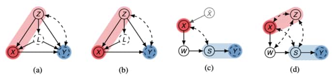
Causal diagrams showing examples where imitation learning can or cannot occur. Blue variables indicate latent reward variable, while red variables represent action. Light red indicates the inputs to the policy space, and light blue represents the minimal imitation surrogates. Figure extracted from [49].

The i-backdoor criterion is used to characterise when imitation of an expert is possible given that the reward variable is unobserved.

Imitation by Backdoor [49]: Given a causal diagram $G$ with policy space $\Pi$, we say that the distribution $P(y)$ is imitable with respect to $\langle G, \Pi \rangle$ if and only if there exists some i-backdoor admissible set $\boldsymbol{Z}$ in this causal system. Further, the policy itself can be determined and is given by $\pi(x \mid pa(\Pi)) = P(x \mid \boldsymbol{z})$.

Applying this theorem, we can see that using set ${Z}$ in the earlier figure (b), an imitating policy is learnable. Further, the policy itself is given by $\pi(x \mid z) = P(x \mid z).$ These results are impressive, but Zhang et al. further point out that the i-backdoor requirement is not necessary for imitation of expert performance. Consider the earlier figure (c) in which variable $S$ mediates all actions (intervention on $X$) on the outcome (latent reward $Y$). We could imagine that learning a distribution over $S$ could be sufficient for imitation of the distribution of $Y$ in this case. This train of thought motivates the following definitions and formalism’s.

Imitation Surrogate [41]: Consider a causal diagram $G$ with policy space $\Pi$. Take $\boldsymbol{S}$ as an arbitrary subset of the observations, $\boldsymbol{O}$. We say $\boldsymbol{S}$ is an imitation surrogate (i-surrogate) with respect to $\langle G, \Pi \rangle$ if $(Y \perp \hat{X} \mid \boldsymbol{S})_{G \cup \Pi}$. Here $G \cup \Pi$ is the graph obtained by adding directed edges from $Pa(\Pi)$ to $X$. $\hat{X}$ is a new parent of $X$ that has been added in this procedure.

We say that the imitation surrogate is minimal if there is no subset of it such that the subset is also an imitation surrogate. A simple example of this is visible in figure (c) where both ${W,S}$ and ${S}$ are surrogates, but ${S}$ is the minimal surrogate. Figure (d) poses an additional problem in that the addition of the collider $Z$ to (c) means $P(s \mid do(\pi))$ is not identifiable even though we have an i-surrogate $S$. The authors tackle this problem by realising that having a subspace of the policy space that yields an identifiable distribution is sufficient to solve the imitation learning task. Without delving into the details here, the authors of [49] implement a confounding robust imitation learning algorithm and apply it to several interesting problems in which the causal approach is shown to be superior to naive imitation learning approaches.

This completes the discussion about this task. I expected causal imitation learning to become an active area of research as this paper was only recently released, being the first of its kind. This also concludes the development of the theory necessary for engaging with state-of-the-art research in causal reinforcement learning.

References

Header Image
[9] Elias Bareinboim. Causal reinforcement learning. ICML 2020, 2020.
[41] M. Kocaoglu, Karthikeyan Shanmugam, and Elias Bareinboim. Experimental design for learning causalgraphs with latent variables. In NIPS, 2017.
[48] P. Abbeel and A. Ng. Apprenticeship learning via inverse reinforcement learning. In ICML ’04, 2004.
[49] J. Zhang, Daniel Kumor, and Elias Bareinboim. Causal imitation learning with unobserved confounders. In June preprint, 2020.

CRL Task 6: Causal Imitation Learning

This Series

Causal Imitation Learning

References

Written by St John Follow