In the previous blog post we discussed and motivated the need for a causal approach to reinforcement learning. We argued that reinforcement learning naturally falls on the interventional rung of the ladder of causation. In this blog post we’ll develop some ideas necessary for understanding the material covered in this series. This might get quite technical, but don’t worry. There is still always something to takeaway. Let’s begin.

This Series

Preliminaries

As you probably recall from high school, probability and statistics are almost entirely formulated on the idea of drawing random samples from an experiment. One imagines observing realisations of outcomes from some set of possibilities when drawing from an assortment of independent and identically distributed (i.i.d.) events. In reality, this assumption of i.i.d. events fails in many situations. Consider shifting some distribution of events or intervening in the system. This failure of an often fundamental assumption in statistics is one reason for the causal approach we shall develop.

In probability theory and statistics, we try to predict an outcome and then associate some probability of an event occurring given some distribution of the underlying space of events. In statistical learning, including machine learning, we are performing the inverse problem. We are trying to find the underlying description of the data. In statistics, the likelihood approach for inference is common for inference. Statistical machine learning can be seen as a simple extension of this approach - applying information gathered from collected data to infer patterns or associations which appear due to the data generating process.

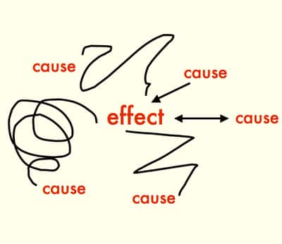
The causal inference and causal learning problem is a harder one. Even if we had perfect and complete knowledge of the observational distribution we would still not know the underlying causal structure of the data.

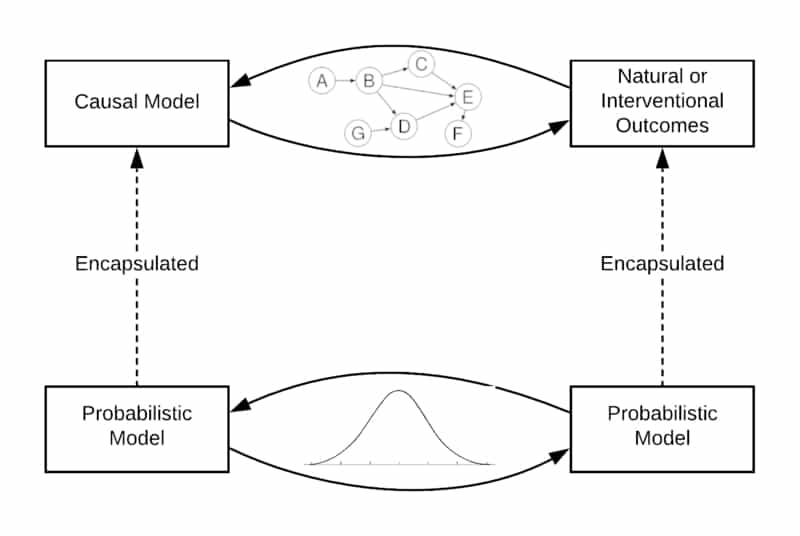
Causal modelling is more fundamental than the probabilistic approach since additional information about relationships between variables is contained in such a model. Causal reasoning allows us to analyse the effects of interventions or distribution changes and make predictions in a more general sense than conventional statistical approaches. Further, it allows for counterfactual reasoning - an ability a reinforcement learning agent generally lacks. Inferring causal structure thus becomes the inverse problem.

Using observational data and outcomes, as well as intervention data, we would like to infer the underlying relationships between the appropriate variables of interest. These relationships between the different modelling and reasoning methods are visualised in the figure below. Although we cannot infer concrete causal structure, we can at least infer the existence of the underlying causal connections from statistical dependence between them. This series of blog posts introduces some advanced theory and techniques for this very subject.

With the preamble done, this section will briefly introduce necessary notions which will either be directly used or helpful in a general context throughout this paper. More detail about basic causal inference theory and reinforcement learning theory is available in the appendices. Perhaps the most fundamental formalism to this formulation of causal theory is the idea of a structural causal model.

Definition (Structural Causal Model (SCM)): A structural causal model \(M\) is a 4-tuple \(\langle U,V,F,P(U) \rangle,\) where

\(U\) are the exogenous variables, determined entirely by external factors
\(V\) are the endogenous variables, determined by other variables in the model.
\(F\) is the set of mappings from \(U\) to \(V\) such that each \(f_i∈F\) maps from \(U_i \cup P_{a_i}\) to \(V_i\) by \(v_i \leftarrow f_i(p_{a_i},u_i)\). Here \(p_{a_i} \in P_{a_i}\), \(U_i \subseteq U\), and \(P_{a_i} \subseteq V\setminus V_i\). In other words, it assigns a value dependent on other variables in the model to a specific variable.
\(P(U)\) is a probability density defined over domain of \(U\).

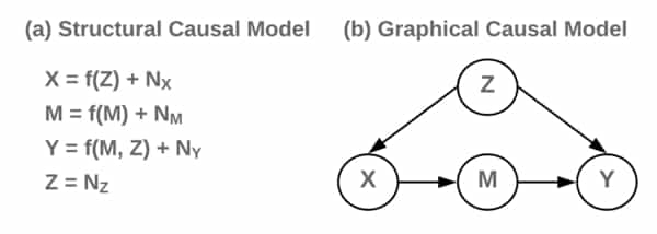
Let’s consider an example. The figure below shows an SCM with an associated graphical representation. Here \(Z\) is exogenous while the other variables are endogenous. Each variable has associated noise variables, \(N\), which indicate the probabilistic nature of the assignments.

Another important concept is that of identifiability. Notice that an SCM induces a joint distribution over the variables of interest. For example, the SCM \(C \rightarrow E\) induces \(P_{C,E}\). Naturally, we wonder whether we can identify, in general, whether the joint distribution came from the model \(C\rightarrow E\) or \(E\rightarrow C\). It turns out we cannot since the graphs are not unique in inducing this joint distribution. In other words, structure is not identifiable from the joint distribution because the underlying graphs add an additional layer of knowledge to the that given by the joint. The proposition below formulates this idea by indicating that we can construct an SCM from a joint distribution in any direction - i.e \(\leftarrow\) or \(\rightarrow\). This is crucial to keep in mind, especially if we plan on trying to use observational data to infer causal structure.

Proposition(Non-uniqueness of graph structures [10]): For every joint distribution \(P_{X,Y}\) of two real-valued variables, there is an SCM \(Y=f_Y(X,N_Y), X⊥Y\), where \(f_Y\) is a measurable function and \(N_Y\) is a real-valued noise variable.

Another important property that will be useful in later analysis is that of d-separation. Essentially, this tells us about the conditional independence relations available in the causal model. In some way, this tells us what information (in the form of variables) ’links’ other variables by way of a causal path. In later sections we will discover this is a very useful property in causal learning and graph manipulation for some important algorithms.

Definition (d-separation [11]): A set \(Z\) of nodes in a causal graph is said to block a path \(p\) if either (1) \(p\) contains at least one incoming or outgoing edge that traverses a vertex in \(Z\), or (2) \(p\) contains at least one collision vertex that is outside \(Z\) and has no descendant in \(Z\). If \(Z\) blocks all available paths from sets \(X\) to \(Y\), the \(X\) and \(Y\) are said to be d-separated by \(Z\).

In the context of causal learning, the d-separation property informs us of how variables are dependent on each other. For example, if \(X\) and \(Y\) are d-separated by \(Z\), we know information cannot travel between \(X\) and \(Y\) by some backdoor if we control for \(Z\). This is a critical notion as it underlies a large portion of this paper dealing with unobserved confounding and latent variables. Another important concept is that of faithfulness.This assumption indicates that causal relations are only formed as a result of d-separation.

The figure above shows examples of causal graphs relating to the theory discussed earlier. (A) shows example of d-separation. (B) shows the resultant graph of an intervention on \(X\), \(do(X=x)\). (C) shows the result of trying to block the direct path between \(X\) and \(Y\) resulting in backdoor paths. Figure extracted from [11].

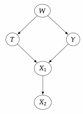
\(d\)-separation is a fundamental idea in modern paradigms of causal inference and very similar ideas will pop up as we consider ideas of causal learning. To reinforce these ideas, let’s consider some examples [14]. In the causal graph below consider the following:

Are \(T\) and \(𝑌\) d-separated by the empty set?
Are \(𝑇\) and \(𝑌\) d-separated by \(𝑊\)?
Are \(𝑇\) and \(𝑌\) d-separated by \(\{𝑊, 𝑋_2\}\)?

To answer these questions, consider the basic building blocks of any causal graph - the chain, fork, and immorality. For chains and forks we can block association between variables by conditioning on the ‘middle’ variable. Notice that by conditioning on the ‘middle’ variable in the immorality we actually open up association between the variables by forcing the value of the parent variables.

In this way, all we have to do to confirm d-separation is make sure we condition on appropriate variables by taking into account these three fundamental graph structures. Let’s work through the first question: Are \(T\) and \(𝑌\) d-separated by the empty set? Notice that \(T \rightarrow X_1 \leftarrow Y\) is an immorality and \(T \leftarrow W \rightarrow Y\) is a fork. Notice that the immorality ensures \(T\) and \(Y\) have no association without conditioning on anything. In other words, having the empty set as our conditioning set. However, this is not true for the fork. There is association by way of the variable \(W\). Thus the empty set \(\{\}\) is not an approapriate conditioning set for d-separation. The next question follows from this logic. Finally, the third question is a little trickier. As a hint, consider what happens to \(X_1\) when we condition on \(X_2\).

Judea Pearl presents three rules of do-calculus that proves sufficient for a wide variety of manipulations between the ’rungs’ on the ladder of causation (see page 234, [7]). The first rule is fairly obvious for the most part. When an observation independent of the variables of interest is made, it does not affect the probability distribution. Formally,

\[P(Y \mid do(X),Z,W)=P(Y \mid do(X),Z)\]

where \(Z\) blocks all paths from \(W\) to \(Y\) in causal model \(G_\overline{X}\). That is, the model with arrows directed into \(X\) removed. The second rule deals with backdoor paths. If \(Z\) satisfies the back-door criterion then \(P(Y \mid do(X),Z) = P(Y \mid X,Z).\) In other words, after controlling for all necessary confounding factors, observation matches intervention. Finally, if there is no causal relationship between \(X\) and \(Y\), then \(P(Y \mid do(X)) = P(Y).\) These three simple rules are remarkably effective in a wide range of proofs. They will prove useful in some examples we discuss in later sections.

Ultimately, we are interested in optimising decision making procedures. The Multi-Armed Bandit (MAB) problem is perhaps the most popular and simplistic setting encountered in literature discussing sequential decision making, and it serves as a key starting point in studies of reinforcement learning (RL). The theory of MAB decision making is also rich and fairly complete for simple scenarios that satisfy strict assumptions. Sutton and Barto [12] - the authors of a seminal introductory text in RL - discuss this problem in detail in the context of optimal control and Bellman optimality.

The MAB problem involves maximising the expected reward/payout given that the reward distribution of each bandit arm is initially unknown to the agent. This can be rephrased as minimisation of the regret the agent experiences, which is the form often encountered in causal and optimal control literature. The regret of a policy or allocation strategy \(A\) after \(n\) plays is defined by

\[\mu^\ast n − \mu_j \sum_{j=1}^K \mathbb{E} [T_j(n)]\]

where \(\mu^\ast = \max_{1 \leq i \leq K} \mu_i.\) Here \(T_i(n)\) denotes the number of times machine ihas been played by policy A, \(\mu\) represents the expected reward of a machine, and \(\ast\) denotes the optimal policy. The regret is thus the expected loss due to sub optimal actions by a policy.

Regret is a natural and intuitive quantity to work with and serves as a proxy for efficiency in learning - key to general intelligence for artificial agents. Regret is a key quantity that this work of causal reinforcement learning addresses. Of course, reinforcement learning is usually interested in sequential decision making over a long-term horizon. This is usually formulated in terms of MDPs.

Definition (Markov Decision Process (MDP) [12]): A Markov decision process (MDP) is a 5-tuple \(\langle S,A,P,R,γ \rangle\) of states \(S\), actions \(A\), transition probabilities \(P\), rewards \(R\), and a discount factor \(\gamma\). Given a state and action, the transition map determines the next state and an associated reward according to the transition probability.

The figure below shows the relationships between variables in a classic RL MDP setting. Clearly the process is Markov in nature. States and rewards are solely based on previous states and taken action. The action is guided by the policy, \(\pi_t\). See [13] for a good introduction to RL.

This MDP model makes several strict, implicit assumptions about the system of interest. For example, that states are fully observed and there is no confounding on any variable of interest. The Markov assumption clearly fails in many areas of interest, including personalised healthcare treatment regimes (dealt with in later sections). This is a key motivator for the need to add causal information to the reinforcement learning theory. We are now ready to begin developing the causal reinforcement learning theory. We start by discussing the context of Bareinboim’s Six Tasks.

The Six Tasks

Causal inference establishes a set of principles and practices for dealing with data from a structural level. Framing the data generating process in causal language while making assumptions about the underlying generative model explicit allows us to reason about causal relationships in a counterfactual nature. Reinforcement learning is concerned with maximising reward in the face of uncertainty in potentially foreign environments and data domains. These two fields, though seemingly disparate, both deal with data in an interventional and - possibly -counterfactual manner. Elias Bareinboim’s CausalAI Lab at Columbia University have sought to tie these fields together by placing them under a single conceptual and theoretical framework [9]. This combination of work has - and is - resulting in powerful results that has not been possible without such an approach. Bareinboim encapsulates the work in this domain as falling under a set of six tasks that these fields can jointly solve and contribute to. He dubs this area of research Causal Reinforcement Learning (CRL). This forms the crux of what this paper investigates, surveys and introduces. It should be noted that Bareinboim et al. are in the process of creating such an introduction to CRL themselves. This paper merely serves to independently survey the field and perhaps provide an alternate context for the framing of this field of work. The interested and motivated reader is encouraged to refer to the source material. Researchers in this area are very active.

We begin by discussing generalised policy learning. In general, this involves systematically combining offline and online modes of observation and interaction (i.e. intervention) with an environment to boost learning performance. We then discuss the problem of identifying when and where to intervene in a causal system. A large portion of this writing is devoted to the third task - counterfactual decision making. This involves exploiting both observational and experimental data to reason about counterfactual quantities and boost learning performance. By leveraging information contained in an agent’s intended action we can learn about unseen factors that are influencing and confounding the system. Next we discuss ideas and methods of learning about structural invariances in a causal system to aid in the transportability of data between domains. The fifth task is focused on learning causal structure from observation and interaction with the environment. Finally, we discuss causal imitation learning. The overall approach to this paper is to include proofs where they aid in explanation or provide important insight into a method or approach to a problem. Additionally, where they demonstrate some useful technique or simply deemed interesting, they will be included. Similarly for placement of figures and included algorithms. This paper is written with brevity in mind, but includes discussion where critical and aids to the overall theme of developing theory for working towards general intelligence. We start by discussing some modern methods for generalising policy learning for a combination of online and offline domains over time horizons that are not necessarily Markov - think healthcare.

References

[8] Elias Bareinboim, Juan D. Correa, Duligur Ibeling, and Thomas Icard. On pearl’s hierarchy andthefoundations of causalinference. unpublished, 2020.
[9] Elias Bareinboim. Causal reinforcement learning. ICML 2020, 2020.
[10] J. Peters, D. Janzing, and B. Schölkopf. Elements of causal inference: Foundations and learning algorithms.2017.
[11] Elias Bareinboim and J. Pearl. Causal inference and the data-fusion problem.Proceedings of the NationalAcademy of Sciences, 113:7345 – 7352, 2016.
[12] Richard Sutton and Andrew Barto.Reinforcement Learning: An Introduction. MIT Press, second editionedition, 2018.
[13] Sergey Levine. Deep rl at berkeley: Cs285. http://rail.eecs.berkeley.edu/deeprlcourse/, 2019.
[14] Brady Neal. Introduction to Causal Inference. https://www.bradyneal.com/causal-inference-course, 2020.

Preliminaries for CRL

This Series

Preliminaries

The Six Tasks

References

Written by St John Follow