In the previous blog post we developed some ideas and theory needed to discuss a causal approach to reinforcement learning. We formalised notions of multi-armed bandits (MABs), Markov Decision Processes (MDPs), and some causal notions. In this blog post we’ll finally get to developing some causal reinforcement learning ideas. The first of which is dubbed Task 1, for CRL can help solve. This is Generalised Policy Learning. Let’s begin.

Generalised Policy Learning

Reinforcement learning typically involves learning and optimising some policy about how to interact in an environment to maximise some reward signal. Typical reinforcement learning agents are trained in isolation, exploiting copious amounts of computing power and energy resources. In a crude manner of speaking, offline policy learning involves learning from a fixed set of collated data. Online policy learning typically involves learning on-the-fly, with the main constraint being time. This approach requires flexibility as data can change over time without any indication of such a change to the agent. In addition, state-of-the-art agents often take a substantial amount of time to train. Transfer learning seeks to solve this inefficiency in the learning process by applying previous knowledge and experience to boost learning performance, similar to how humans can exploit previous knowledge to solve novel tasks. The field of causal inference similarly deals with this problem of inferring effect from heterogeneous sources of data. A major problem in this process involves learning in the face of unobserved (hidden) confounders. We now discuss some ideas of how causal inference and modelling can be applied to multi-armed bandits (MABs) and Markov decision processes (MDPs) to boost learning performance by combining different modes of learning - observation and interventional.

One such paper that tackles this problem is ¹Zhang, J., & Bareinboim, E. (2017). Transfer learning in multi-armed bandits: A causal approach. IJCAI-17:1340–1346. in which the authors combine transfer learning in (basic) reinforcement learning with causal inference theory. This is done in the context of two multi-armed bandit agents given access to a causal model of the environment. In the case where causal effects are not identifiable, the authors provide a method of extracting causal bounds from available knowledge contained in the available distributions. We now develop some of the theory presented in this paper.

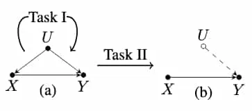
Contextual bandits are discussed in ²Langford, J., & Zhang, T. (2007). The epoch-greedy algorithm for contextual multi-armed bandits. NIPS. and are a variation of MABs such that the agent can observe additional information (context) associated with the reward signal. The authors of ¹Zhang, J., & Bareinboim, E. (2017). Transfer learning in multi-armed bandits: A causal approach. IJCAI-17:1340–1346. start by considering an off-policy learning problem such that agent $A$ follows some policy $do(X = \pi(\epsilon, u))$ with context $u \in U$ and noise $\epsilon$, resulting in joint distribution $P(x,y,u)$. Another agent, $A^\prime$, would similarly like to learn about the environment and exploit the experience of $A$ to boost its learning and quickly converging upon the optimal policy. This problem boils down to identifying the causal effect of an intervention on $X$, given by $\mathbb{E}[Y \mid do(x)]$. That is, the expected outcome given that we experiment by intervening on $X$. A more challenging scenario appears if we wish to transfer knowledge from this contextual bandit to a standard MAB agent, say $B$ (see figure below). If we denote by $G_{\overline{X}\underline{Z}}$ the subgraph obtained by deleting all edges directed into $X$ and all edges directed out of $Z$, then $(Y \perp X \mid U)_{\underline{G}}$ means that by removing edges directed out of G, given the context $U$, we obtain that $Y$ is independent of $X$. This is useful because we can then derive $\mathbb{E}[Y \mid do(x)] = \sum_{u \in D(U)} \mathbb{E}[Y \mid x, u] P(u)$ (applying the second rule of $do$-calculus). In this case the average effect $\mathbb{E}[Y \mid do(x)]$ was identifiable - there were not multiple causal structures inducing the same distribution. The authors note that $do$-calculus provides a complete method for identifying such causal effects but it is not useful for constructing such formulae for non-identifiable queries. For example, if agent $B$ cannot observe the context in which $A$ operates, $do$-calculus cannot identify the average effect $\mathbb{E}[Y \mid do(x)]$ since different causal models can induce the same observational distribution $P(x,y)$ with different expected rewards. This is a very important concept to note since naivete in the transfer process under these conditions can lead to negative impact on the performance of the target. In practice, however, we often don’t have access to the underlying SCMs beforehand, and thus cannot distinguish between two such models.

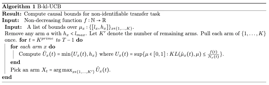
At this point it is natural to assume that if the identifiability condition does not hold then prior data is not useful in the transfer process. Remarkably though, ¹Zhang, J., & Bareinboim, E. (2017). Transfer learning in multi-armed bandits: A causal approach. IJCAI-17:1340–1346. shows that for non-identifiable tasks we can still obtain causal bounds over the expected rewards of the target agent. This is achieved by using prior knowledge to construct a general SCM compatible with all the available models. Let us consider this is some detail. Given an stochastic MAB problem such that it has a prior represented as a list of bounds over the expected rewards, then for any bandit arm $x$, let $\mu_x \in [l_x,h_x]$. WLOG, assume $0 < l_x < h_x < 1$ and denote $l_{max} = \max_{x = 1, \dots, K} l_x$. Note that a K-MAB problem is simply a generalisation of the MAB problem to multiple independent bandits. The following theorem is presented and proved by the authors:

Theorem: Consider a K-MAB problem with rewards bounded in $[0,1]$, with each arm $x \in \{ 1, \dots, K \}$, and expected reward $\mu_x \in [l_x,h_x]$ s.t. $0 < l_x < h_x < 1$. Taking $f(t) = \log(t) + 3\log(\log(t))$, in the B-kl-UCB algorithm (shown in algorithm below), the number of draws of $\mathbb{E}[N_x(T)]$ for any sub-optimal arm $a$ is upper bounded for any horizon $T \geq 3$ as:

$$\left\{\begin{array}{ll} 0 & \text {if } h_{x}<l_{\max } \\ 4+4 e \log (\log (T)) & \text {if } h_{x} \in\left[l_{\max }, \mu^{*}\right) \\ \frac{\log (T)}{K L\left(\mu_{x}, \mu^{*}\right)}+\mathcal{O}\left(\frac{\log (\log (T))}{K L\left(\mu_{x}, \mu^{*}\right)}\right) & \text { if } h_{x} \geq \mu^{*} \end{array}\right.$$

Though seemingly very abstract, this theorem tells us that if the causal bounds impose strong constraints over the arm’s distribution then the B-kl-UCB algorithm (see below) provides asymptotic improvements over its unbounded counterpart (the kl-UCB algorithm ³Garivier, A., & Cappé, O. (2011). The KL-UCB algorithm for bounded stochastic bandits and beyond., not presented here). This implies that constraints translate into different regret bounds for the MAB agent. We could expect that finding such constraints over our problem bounds would increase performance. The algorithm below should be self-contained. For more information refer to the source material.

Zhang and Bareinboim ⁴Zhang, J., & Bareinboim, E. (2019). Near-optimal reinforcement learning in dynamic treatment regimes. NeurIPS. extend similar ideas to the field of dynamic treatment regimes (DTRs) and personalised medicine. A DTR consists of a set of decision rules controlling the provided treatment at any given stage, given a patient’s conditions. The challenge is to apply online reinforcement learning algorithms to the problem of selecting optimal DTRs given observational data, with the hope that RLs sample efficiency success in other decision making processes can translate to DTRs. Policy learning in this case refers to the process of finding an optimal policy $\pi$ that maximises some outcome $Y$ - usually the patient’s recovery or improvement in health markers. Often, however, the parameters of the DTR remain unknown and direct optimisation isn’t possible. Traditional algorithms rely on there being no unobserved confounders, while randomisation techniques are often not feasible in the medical domain. We certainly wouldn’t want doctors randomly testing strategies on patients to see ‘how it plays out’! Reinforcement learning offers an attractive set of techniques for DTRs as it should offer an efficient means to learn DTRs while balancing the exploration of state-space and exploitation of rewards. Existing RL techniques, however, are not applicable in the DTR context as they rely on the Markov property. DTRs are clearly non-Markovian as the treatment procedure at some point in the future is a function of past treatments. The authors formalise this in causal language as follows:

Dynamic Treatment Regime: A dynamic treatment regime (DTR) is a SCM $\langle \boldsymbol{U}, \boldsymbol{V}, \boldsymbol{F}, P(\boldsymbol{u}) \rangle$ where the endogenous variables $\boldsymbol{V} = \{ \overline{\boldsymbol{X}}_K, \overline{\boldsymbol{S}}_K, Y \}$ are the total stages of interventions. Here $\overline{\boldsymbol{X}}_K$ represents a sequence $\{X_1,\dots,X_K\}$. Values of exogenous variables $\boldsymbol{U}$ are drawn from the distribution $P(\boldsymbol{u})$. For stage $k = 1, \dots, K:$

1. $X_k$ is a finite decision decided by a behaviour policy $x_k \leftarrow f_k(\overline{\boldsymbol{s}}_k, \overline{\boldsymbol{x}}_{k-1}, \boldsymbol{u})$.
2. $S_k$ is a finite state decided by a transition function $s_k \leftarrow \tau_k(\overline{\boldsymbol{x}}_{k-1}, \overline{\boldsymbol{s}}_{k-1}, \boldsymbol{u})$.
3. $Y$ is the primary outcome at the final state $K$, decided by a reward function $y \leftarrow r(\overline{\boldsymbol{x}}_{K}, \overline{\boldsymbol{s}}_{K}, \boldsymbol{u})$ bounded in $[0,1]$.

A DTR $M^\ast$ induces some observational distribution $P(\overline{\boldsymbol{x}}_{K}, \overline{\boldsymbol{s}}_{K}, \boldsymbol{u}))$, responsible for the data we observe without intervention. A policy $\pi$ for the DTR defines some sequence of stochastic interventions $do(X_1 \sim \pi_1(X_1 \mid \overline{\boldsymbol{S}_1}), \dots, \pi_K(X_K \mid \overline{\boldsymbol{S}}_K, \overline{\boldsymbol{X}}_{K-1}))$. These interventions induce an interventional distribution $P_{\pi}\left(\overline{\boldsymbol{x}}_{K}, \overline{\boldsymbol{s}}_{K}, y\right)=P_{\overline{\boldsymbol{x}}_{K}}\left(y \mid \overline{\boldsymbol{s}}_{K}\right) \prod_{k=0}^{K-1} P_{\overline{\boldsymbol{x}}_{k}}\left(s_{k+1} \mid \overline{\boldsymbol{s}}_{k} \right) \pi_{k+1}\left(x_{k+1} \mid \overline{\boldsymbol{s}}_{k+1}, \overline{\boldsymbol{x}}_{k}\right),$ where $P_{\overline{\boldsymbol{x}}_{k}}\left(s_{k+1} \mid \overline{\boldsymbol{s}}_{k} \right)$ is the transition distribution at stage $k$, and $P_{\overline{\boldsymbol{x}}_{K}}$ is the reward distribution over the primary outcome. The expected cumulative reward is then $V_\pi(M^\ast) = \mathbb{E}_{\pi}[Y]$, implying our task is to find $\pi^\ast = \textbf{argmax}_{\pi \in \Pi} V_{\pi}(M^\ast).$ In other words, we would like to find the policy that finds the best sequence of actions that leads to an optimal outcome. The notation $V_\pi$ is deliberately chosen to correspond to value functions in RL literature.

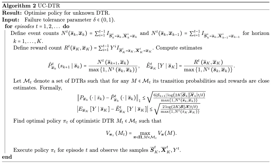
The authors introduce the UC-DTR algorithm, presented in the algorithm below, to optimise an unknown DTR. This algorithm takes an optimism in the face of uncertainty approach - a common strategy in the reinforcement learning literature. Given only knowledge of the state and action domains, UC-DTR achieves near-optimal total regret bounds. This is really quite remarkable. Knowing only about the current state and the possible actions we can take, we have an algorithm to reach almost optimal outcomes in very few steps! We now delve into the algorithm a bit deeper and discuss the overall strategy it employs. First, a new policy $\pi_t$ is proposed using samples

$\{ \overline{\boldsymbol{S}}_K^i, \overline{\boldsymbol{X}}_K^i, Y^i \}_{i=1}^{t-1}$

collected up until the current episode, $t$. That is, the deciding agent exploits its current knowledge to propose what it believes to be a good policy choice. The empirical estimates for the expected reward and the transitional probabilities are calculated and used to consider a set of plausible DTRs in terms of a confidence region around these estimates. The optimal policy of the most optimistic DTR in the plausible DTR set is calculated and executed to collect the next set of samples. This is the optimism and the uncertainty we discussed earlier. This procedure is repeated until a tolerance level or specific episode is reached. The authors proceed to show that the the UC-DTR algorithm has cumulative regret that scales with

$\tilde{\mathcal{O}}(K\sqrt{|\mathcal{\boldsymbol{S}}||\mathcal{\boldsymbol{X}}|T}),$

where $\tilde{\mathcal{O}}(\cdot)$ is like Big-Oh notation but also ignores $\log$-terms. Formally,

$f = \tilde{\mathcal{O}}(g) \Leftrightarrow \exists k, f = \mathcal{O}(g \log^k(g)).$

The proofs for this analysis are fairly involved and are provided in the appendix of ⁴Zhang, J., & Bareinboim, E. (2019). Near-optimal reinforcement learning in dynamic treatment regimes. NeurIPS..

Theorem: Fix tolerance parameter $\delta \in (0,1)$. With probability at least $1 - \delta$, it holds for any $T > 1$ that the regret of UC-DTR is bounded by

$R(T) \leq 12 K \sqrt{|\mathcal{S}||\mathcal{X}| T \log (2 K|\mathcal{S}||\mathcal{X}| T / \delta)}+4 K \sqrt{T \log (2 T / \delta)}.$

Theorem: For any algorithm $\mathcal{A}$, any natural numbers $K \geq 1$, and

$|\boldsymbol{\mathcal{S}}^k| \geq 2 \quad\text{and}\quad |\boldsymbol{\mathcal{X}}^k| \geq 2$

for any $k \in \{ 1, \dots, K \}$, there is a DTR $M$ with horizon $K$, state domains $\boldsymbol{\mathcal{S}}$ and action domain $\boldsymbol{\mathcal{X}},$ such that the expected regret of $\mathcal{A}$ after

$T \geq |\boldsymbol{\mathcal{S}}||\boldsymbol{\mathcal{X}}| \quad\text{episodes is at least}\quad \mathbb{E}[R(T)] \geq 0.05 \sqrt{|\boldsymbol{\mathcal{S}}||\boldsymbol{\mathcal{X}}| T}.$

Together, these theorems indicate that UC-DTR is near-optimal given only the state and action domains. The authors further propose exploiting available observational data to improve performance of the online learning procedure in the face of unobserved confounders and non-indentifiability. Using observational data, the authors derive theoretically sound bounds on the the system dynamics in DTRs. We include the full UC-DTR algorithm below as it is indicative of a general algorithmic approach to similar problems in the causal reinforcement literature. The reader is encouraged to work through the steps to confirm that it matches the theory discussed above. The explanations for the steps are fairly self-contained and are not discussed further for brevity.

We have discussed some interesting theory that underlines much of the later work in this active area of research. The interested reader is encouraged to refer to ⁵Zhang, J., & Bareinboim, E. (2020). Designing optimal dynamic treatment regimes: A causal reinforcement learning approach. ICML. for extensions to dynamic treatment regimes. ⁶Namkoong, H., Keramati, R., Yadlowsky, S., & Brunskill, E. (2020). Off-policy policy evaluation for sequential decisions under unobserved confounding. and ⁷Zhang, J., & Bareinboim, E. (2020). Bounding causal effects on continuous outcomes. will interest the readers motivated by the development of further theory for generalised decision making and performance bounding. We are now ready to discuss the problem of finding where in a causal system we should intervene for optimal and efficient outcomes.

References

1. Zhang, J., & Bareinboim, E. (2017). Transfer learning in multi-armed bandits: A causal approach. IJCAI-17:1340–1346.
2. Langford, J., & Zhang, T. (2007). The epoch-greedy algorithm for contextual multi-armed bandits. NIPS.
3. Garivier, A., & Cappé, O. (2011). The KL-UCB algorithm for bounded stochastic bandits and beyond.
4. Zhang, J., & Bareinboim, E. (2019). Near-optimal reinforcement learning in dynamic treatment regimes. NeurIPS.
5. Zhang, J., & Bareinboim, E. (2020). Designing optimal dynamic treatment regimes: A causal reinforcement learning approach. ICML.
6. Namkoong, H., Keramati, R., Yadlowsky, S., & Brunskill, E. (2020). Off-policy policy evaluation for sequential decisions under unobserved confounding.
7. Zhang, J., & Bareinboim, E. (2020). Bounding causal effects on continuous outcomes.

Comments are being migrated. Check back soon.