In the previous blog post we discussed the gorey details of generalised policy learning - the first task of CRL. We went into some very detailed mathematical description of dynamic treatment regimes and generalised modes of learning for data processing agents. The next task is a bit more conceptual and focuses on the question on how to identfy optimal areas of intervention in a system. This is clearly very important for an RL agent where its entire learning mechanism is based on these very interventions in some system with a feedback mechanism. Let’s begin!

This Series

Interventions - When and Where?

A classic problem in reinforcement learning literature regards the trade-off between exploration of the state-action space, to test interventional outcomes over a long-term horizon, and weigh this against greedy exploitation of current knowledge of the behaviour of the underlying causal system. The multi-armed bandit (MAB) problem is a classic setting for the study of decision making agents - a situation where long-term planning is not required. Recent literature has placed focus on the effect of non-trivial dependencies amongst arms of the bandits, referred to as structural bandits. Researchers interested in causal reasoning have experimented and investigated modelling some of these dependencies with causal graph structures. For example, [21] discusses reinforcement learning in the context of causal models with unobserved confounders. This is discussed in detail in the next blog of this series, with key insight being that counterfactual quantities can aid in taking into account unobserved confounders. In this setting, traditional methods do not guarantee convergence to a reasonable policy while counterfactual-aware methods can make this guarantee. The goal of this section is to identify the optimal action an MAB should take where the arm of the MAB corresponds to an intervention on some causal graph. In this way we hope to use knowledge of causal systems to identify theoretically optimal interventional decisions. To discuss MAB instances in the context of causal inference, we now formalise the notion of an SCM-MAB.

Structural Causal Model - Multi-Armed Bandit (SCM-MAB) [22] Let $M$ be a SCM $\langle \boldsymbol{U}, \boldsymbol{V}, \boldsymbol{F}, P(\boldsymbol{U}) \rangle$ and $Y \in \boldsymbol{V}$ be a reward variable with domain $\mathbb{R}$. The arms of the bandit are such that ${ \boldsymbol{x} \in Dom(\boldsymbol{X}) \mid \boldsymbol{X} \subseteq \boldsymbol{V} \setminus {Y} }$. In other words, the arms are the set of possible interventions on all the endogenous variables of the SCM, excluding the reward. Each arm of the MAB is associated with a reward interventional distribution $P(Y \mid do(x))$, having mean $\mu_x = \mathbb{E}[Y \mid do(x)].$

We assume the SCM-MAB has knowledge of the underlying causal graph and reward, but does not know about the SCM mappings $\boldsymbol{F}$, or the joint distribution over the exogenous variables $P(\boldsymbol{U})$. Recall, we are interested in finding a minimal set of interventions that optimises the actions. This motivates the following definitions. Here, we denote the information gained by an agent interacting with the SCM-MAB by $[[ G, Y ]]$.

Minimal Intervention Set (MIS) [22]: A set of endogenous variables $\boldsymbol{X} \subseteq \boldsymbol{V} \setminus {Y}$ is said to be a minimal intervention set relative to $[[ G, Y ]]$if $\not\exists \boldsymbol{X}^\prime \subset \boldsymbol{X}$ such that $\mu_{x^\prime} = \mu_x$ where $x^\prime \in \boldsymbol{X^\prime}$ for every SCM complying with the causal structure dictated by the causal graph. In other words, there is no intervention set smaller than the proposed set that results in the same mean reward.

Thinking about the definition, we realise that by intervening on the ancestors of the reward variable, $Y$, is a sufficient and necessary condition for a MIS.

Minimality [22]: A set of endogenous variables $\boldsymbol{X} \subseteq \boldsymbol{V} \setminus {Y}$ is a MIS for the causal graph G and reward variable $Y$ if and only if $\boldsymbol{X} \subseteq an(Y){G{\overline{X}}}.$

This proposition provides a method for finding the MISs given the information available to the agent. We can simply pass over all the possible subsets of the endogenous variables $\boldsymbol{X} \setminus {Y}$ and check the proposition. Of course, based on the structure of causal graphs, it is possible that intervening on one set of variables is always superior to intervening on another. This induces a partial ordering: given two sets of variables $\boldsymbol{W}, \boldsymbol{Z} \subseteq \boldsymbol{V} \setminus {Y}$ such that $\max_{\boldsymbol{w}\in Dom(\boldsymbol{W})} \mu_{\boldsymbol{w}} \leq \max_{\boldsymbol{z}\in Dom(\boldsymbol{Z})} \mu_{\boldsymbol{z}}$ in all the possible SCMs that comply with the rules defined by the causal graph, then we have a method of comparing the preferable intervention sets. This motivates the need to formalise the notion of a possibly optimal MIS.

Possibly-Optimal MIS (POMIS) [22]: Given information $[[ G, Y ]]$ and MIS $\boldsymbol{X}$. If there exists a SCM following rules defined by causal graph $G$ and $\mu_{\boldsymbol{x}^\ast} > \mu_{\boldsymbol{z}^\ast} \forall {\boldsymbol{Z} \in \mathbb{Z} \setminus {\boldsymbol{X}}}$, we say $\boldsymbol{X}$ is a possibly optimal MIS. Here $\mathbb{Z}$ represents the possible MISs complying with $G$ and $Y$.

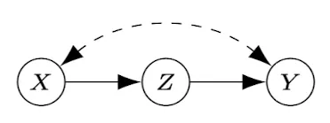
One key assumption we have made is that any observed variable can be intervened on. This is, of course, a ludicrous assumption to be made in general, and the studying of the relaxed condition becomes relevant for general application of these techniques. [23] investigates identifying possibly-optimal arms in the structural causal bandit framework when only partial causal knowledge is available and select variables are not manipulable. Take a look at the figure above and notice that according to the POMIS definition, intervening on $Z$ is possibly optimal. If intervening on this variable is not feasible (i.e. non-manipulable) then we should consider $X$ to be possibly optimal instead. Of course, we could have that not intervening at all ($do(\theta)$) is optimal. We can augment the definitions of MIS and POMIS by replacing the endogenous variables under consideration, $\boldsymbol{X} \subseteq \boldsymbol{V} \setminus {Y}$ with $\boldsymbol{X} \subseteq \boldsymbol{V} \setminus {Y} \setminus \boldsymbol{N}$, where $\boldsymbol{N}$ represents the variables that are non-manipulable in the causal system. For brevity we do not formalise this as it follows directly by augmenting previous definitions.

Identifying all the POMIS given that we have $\boldsymbol{N} \neq \theta$ (i.e. there are non-manipulable variables) is non-trivial because simply removing intervention sets that contain manipulable variables will not necessarily be exhaustive of the possibly-optimal sets. If this is not clear, refer back to the figure above and notice that the possibly-optimal set ${X}$ (when $Z$ is non-manipulable) would not be identified in this case. This motivates the need for new techniques. The root of the problem is that there is a possibility for a POMIS to exist that would not be a POMIS in the unconstrained case. The idea presented in [17] is to project the constrained graph onto a subgraph containing only unconstrained variables, and then identify the (unconstrained) POMIS structures in this realm. We now describe the method [17] presents to project a constrained causal graph onto the unconstrained graph, ready for POMIS identification.

Initialise graph $H = \langle \boldsymbol{V} \setminus \boldsymbol{N}, \theta \rangle$.
Add edge $V_i \rightarrow V_j$ if there exists path $V_i \rightarrow V_j$ in the original causal graph $G$; or
Add edge $V_i \rightarrow V_j$ if there exists a directed path from $V_i$ to $V_j$ where all intermediate nodes are in $\boldsymbol{N}$.
Similarly, add edge $V_i \leftrightarrow V_j$ if there exists path $V_i \leftrightarrow V_j$ in the original causal graph; or
Add edge $V_i \leftrightarrow V_j$ if there exists a bidirected (unobserved confounder) path from $V_i$ to $V_j$ where all intermediate nodes are in $\boldsymbol{N}$.

Figure \ref{fig:ZB-2019-Fig4} displays some examples of this projection procedure for removing different variables. The authors proceed to show that this projection is guaranteed to preserve the POMISs, and that the underlying SCMs of both graphs (original and projected) maintain the same observational and interventional distributions. By applying these techniques to simulated datasets, the authors show that the POMIS technique significantly outperforms brute-force intervention techniques and simpler MIS identification to identify optimal arm selection. They also experiment with adding $z$-identifiability (discussed in later sections) to the POMIS method, which improves it further.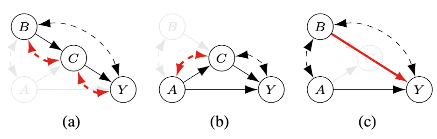

In this section we have briefly discussed some graphical criteria and procedures for identifying optimal sets of variables to intervene on. [24] extend these ideas to identifying optimal intervention variables in mixed policies - cases where both observational and interventional information is available. The reader is encouraged to refer to this paper. One key idea presented in work in this area is that of $z$-identifiability which encapsulates the idea of what we can learn by intervening on variables in the causal system. This idea is generalised in later sections (see task 4). This leads well to the next section which discusses a key theme in this paper - counterfactual decision making.

References

[17] J. Zhang and Elias Bareinboim. Near-optimal reinforcement learning in dynamic treatment regimes. In NeurIPS, 2019.
[21] Elias Bareinboim, Andrew Forney, and J. Pearl. Bandits with unobserved confounders: A causal approach. In NIPS, 2015.
[22] Sanghack Lee and Elias Bareinboim. Structural causal bandits: Where to intervene? In NeurIPS, 2018.
[23] Sanghack Lee and Elias Bareinboim. Structural causal bandits with non-manipulable variables. In AAAI,2019.
[24] S. Lee. Characterizing optimal mixed policies: Where to intervene and what to observe. 2020.

CRL Task 2: Interventions - When and Where?

This Series

Interventions - When and Where?

References

Written by St John Follow

References

- Bareinboim, E., Forney, A., & Pearl, J. (2015). Bandits with unobserved confounders: A causal approach. NIPS.
- Lee, S., & Bareinboim, E. (2018). Structural causal bandits: Where to intervene?. NeurIPS.
- Lee, S., & Bareinboim, E. (2019). Structural causal bandits with non-manipulable variables. AAAI.
- Zhang, J., & Bareinboim, E. (2019). Near-optimal reinforcement learning in dynamic treatment regimes. NeurIPS.
- Lee, S. (2020). Characterizing optimal mixed policies: Where to intervene and what to observe.
Comments are being migrated. Check back soon.