We’ve now come to one of the most vital aspects of this theory - how can we learn causal models? Learning models is often an exceptionally computationally intensive process, so getting this right is crucial. We now develop some mathematical results which guarantee bounds on our learning. We’ll start by discussing the current state of this field in relation to causal inference and reinforcement learning.

Learning Causal Models

Perhaps one of the most computationally difficult processes in the field of causal inference is that of learning underlying causal structure by algorithmically identifying cause-effect relationships. In recent years there has been a surge of interest in learning such relationships in the fields of machine learning and artificial intelligence, though it has been relatively prevalent in the social sciences for many years now (e.g. ¹Granger, C. W. J. (1969). Investigating causal relations by econometric models and cross-spectral methods. Econometrica 37:424–438. has over 25000 citations at time of writing). The discovery of IC and PC ²Spirtes, P., Glymour, C., & Scheines, R. (2000). Causation, Prediction, and Search (2nd ed.). Adaptive Computation and Machine Learning. algorithms independently displayed the feasibility of learning such causal structure from observational data - a fact that was not obvious at the time. Since these discoveries new methods of inferring such structure have emerged. Many of these methods require satisfaction of the strict causal sufficiency assumption. This requires that no latent variables affects more than one observed variable. In other words, these algorithms do not deal with confounding.

³Kocaoglu, M., Shanmugam, K., & Bareinboim, E. (2017). Experimental design for learning causal graphs with latent variables. NIPS. improves upon previous work by introducing an algorithm that can learn any causal graph, as well as the existence and location of the latent variables using $\mathcal{O}(d\log(n) + l)$ interventions, where $d$ is the largest node degree, and $l$ is the longest directed path of the causal graph. Further, they introduce a probabilistic algorithm which can learn the observable graph and all the latent variables using $\mathcal{O}(d\log^2(n) + d^2\log(n))$ interventions with high probability. We discuss and develop this theory as it is deemed a particularly interesting approach to the problem at hand. The authors split the task of learning the observable graph and latent variables into three distinct sub-tasks. They start by proposing a method for finding the transitive closure of the observable graph. Next, this transitive closure is reduced to reveal some subset of the edges in the underlying causal graph. Conditional independence tests are then used to uncover latent variables. We now discuss select theory in detail.

The authors begin by showing that separating systems can be used to construct sequences of pairwise conditional independence tests to discover the transitive closure of the observable causal graph. That is, to discover the causal paths in the causal system by testing which variables ‘rely’ on other variables (in an informal sense). To develop this idea formally we require the idea of a post-interventional causal graph. This is simply the causal graph $G$ with all edges directed onto intervened variables, removed. Recall that faithfulness indicates that causal relations are only formed as a result of d-separation. Simply put, there are no relationships that perfectly balance each other so as to appear to have no causal relations. These conditions allow us to formalise the conditional independence test we require.

Pairwise Conditional Independence Test ³Kocaoglu, M., Shanmugam, K., & Bareinboim, E. (2017). Experimental design for learning causal graphs with latent variables. NIPS.: Consider causal graph with latent variables $D_l$, and an intervention set $S \subset V$ of observable variables. Applying the post-interventional faithfulness assumption, we have that for any pair $X_i \in S, X_j \in V \setminus S, (X_i \not\perp X_j)_{D_l[S]}$ if and only if $X_i$ is an ancestor of $X_j$ in the post-interventional graph $D[S].$

This lemma provides a method for determining ancestry for any ordered pair of variables, $(X_i, X_j).$ Crucially though, this method is not sufficient. For example, consider $X_i \rightarrow X_k \rightarrow X_j$ where $X_i,X_k \in S, X_j \not\in S.$ The authors propose resolving this issue by using a sequence of interventions guided by a separating system. The correct causal graph can then be learned by finding the transitive closure.

$(m,n)$ Strongly Separating System ³Kocaoglu, M., Shanmugam, K., & Bareinboim, E. (2017). Experimental design for learning causal graphs with latent variables. NIPS.: An $(m,n)$ strongly separating system is a collection of subsets $\{ S_1, S_2, \dots, S_m \}$ of the ground set $[n]$ such that for any two pairs of nodes $i$ and $j$, there exists a set $S$ in the family such that $i \in S, j \not\in S$ and also another set $S'$ such that $i \not\in S', j \in S'$.

This definition is useful because, as shown in ³Kocaoglu, M., Shanmugam, K., & Bareinboim, E. (2017). Experimental design for learning causal graphs with latent variables. NIPS., a strong separating system always exists on ground set $[n]$ when $m \leq 2 \lceil \log n \rceil$. This allows us to introduce a deterministic algorithm for learning the observable causal graph $D$ from the ancestral relationships, which requires only $2 \lceil \log n \rceil$ interventions and conditional independence tests. A key insight for the deterministic algorithm is that whenever the intervention set contains all parents of $X_i$, the only variables that are dependent with $X_i$ in the post-interventional set are the parents, $Pa_i$. Consider $r$, the longest directed path of $D_{tc}$. Using the obvious partial order $<_{D_{tc}}$ on the vertex set $V$, we can define a unique partitioning of vertices $\{ T_i \mid i \in [r + 1] \}$ where $T_i <_{tc} T_j \forall i<j$. Each node in $i$ is thus a set of of mutually incomparable elements and represents the set of nodes at layer $i$ in the transitive closure graph $D_{tc}$. Define $\mathcal{T}_{i} = \cup_{k=1}^{i-1} T_k$, then $Pa_i \subset T_i$ - a fact that is exploited for the deterministic algorithm the authors present.

Perhaps the most interesting aspect of this paper is the randomised algorithm the authors propose. The strategy employed here is to repeatedly use the ancestor graph learning algorithm to learn the observable graph. This procedure makes use of transitive reduction.

Transitive Reduction: Given a directed acyclic graph $D = (V,E)$, let its transitive closure be $D_{tc}.$ Then $Tr(D) = (V, E_r)$ is a directed acyclic graph with minimum number of edges such that its transitive closure is identical to $D_{tc}$.

This transitive reduction is simple and effective. This allows for an iterative procedure for revealing causal relationships. We now elaborate on this procedure in the following lemma, discussed in ³Kocaoglu, M., Shanmugam, K., & Bareinboim, E. (2017). Experimental design for learning causal graphs with latent variables. NIPS..

Lemma: Given intervention set $S \subset V$ of nodes in the observable causal graph $D$, we can notate the post-interventional observable causal graph as $D[S]$. Now, consider a specific observable node $V_i \in S^C$, and let $Y$ be a direct parent of $V_i$ in $D$ such that all the direct parents of $V_i$ above $Y$ in the partial order $\pi(\dot)$ are in $S$. Formally, $\{ X \mid \pi(X) > \pi(Y), (X,V) \in D \} \subseteq S$. Then $Tr(D[S])$ will contain the directed edge $(Y,V_i)$ and it can be computed from $Tr((D[S])_{tc})$.

To solidify the simplicity of the lemma, consider the figure below. Here we show how an intervention changes what the procedure can reveal about the structure of the transitive relationships in the observable causal graph.

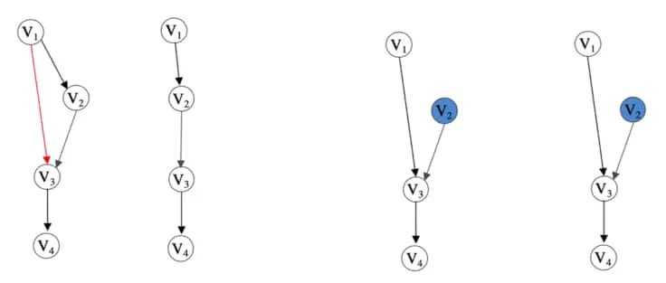
Figure showing examples of theory in ³Kocaoglu, M., Shanmugam, K., & Bareinboim, E. (2017). Experimental design for learning causal graphs with latent variables. NIPS.. Starting from the left, we have an example of a graph without latent variables. Next, we have the result of the transitive reduction procedure on the previous graph. Notice that the red edge has not been revealed. Next, we have the same observational graph but with $V_2$ intervened on. This removes the direct causal relation between $V_1$ and $V_2$ and thus reveals edge $V_1 \rightarrow V_3$ in the transitive reduction procedure (shown last). Figure extracted from ³Kocaoglu, M., Shanmugam, K., & Bareinboim, E. (2017). Experimental design for learning causal graphs with latent variables. NIPS..

This procedure is useful for the probabilistic algorithm the authors propose. Here, the basic idea is that random intervention and transitive closure computation can reveal edges of the underlying causal graph. As we perform more interventions, our certainty about the structure of the observable causal graph rises. The following theorem ³Kocaoglu, M., Shanmugam, K., & Bareinboim, E. (2017). Experimental design for learning causal graphs with latent variables. NIPS. formalises this idea.

Theorem: Let $d_{max}$ exceed the the maximum in-degree in the observable graph $D$. The proposed probabilistic algorithm requires at most $8cd_{max}(\log n)^2$ interventions and conditional independence tests on samples obtained from post-interventional distributions, and returns the observable portion of the causal graph with a minimum probability of $1-\frac{1}{n^{c-2}}$.

We now consider a more involved scenario. Recall that conditioning on an observable is not necessarily sufficient due to backdoor paths. Consider the scenarios in the figure below. On the left, we have an example of a graph where intervening on $X$ leaves an influencing path open, $X \leftarrow U \rightarrow T \leftarrow M \rightarrow Y$. This means that observation does not necessarily match our intervention data, $P(Y \mid X) \neq P(Y \mid do(X))$. We must intervene on a parent of $X$ to remove confounding influences in this example. Similarly for the graph on the right where we need to intervene on parents of $Y$. This motivates the following theorem.

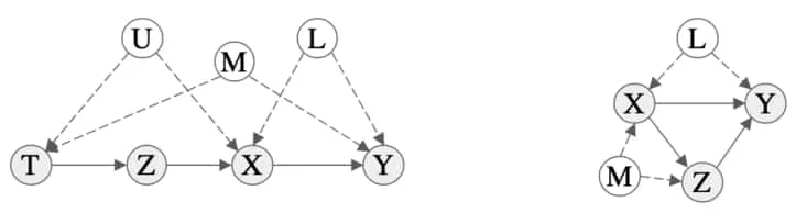
Figure showing examples of graphs that require a more complex intervention to block backdoor paths. Details about these are discussed in the text. Figure extracted from ³Kocaoglu, M., Shanmugam, K., & Bareinboim, E. (2017). Experimental design for learning causal graphs with latent variables. NIPS..

Interventional Do-See Test ³Kocaoglu, M., Shanmugam, K., & Bareinboim, E. (2017). Experimental design for learning causal graphs with latent variables. NIPS.: Given a causal graph $G$ over observable variables $V$ and latents $L$. Denoting edge set of $G$ by $E$, then

$P(V_j \mid V_i = v_i, do(Pa_i = pa_i, Pa_j = pa_j))$

$= P(V_j \mid do(V_j \mid do(V_i = v_i, Pa_i = pa_i, Pa_j = pa_j))),$

if and only if there exists some $k \in \mathbb{N}$ such that $(L_k, V_i) \in E$ and $(L_k, V_j) \in E$. Recall, $Pa_i$ are the parents of $V_i$.

The final result of this paper is, perhaps, the most mathematically satisfying and, otherwise, surprising. We will need some theory of graph colourings to present this.

Strong Edge Colouring ³Kocaoglu, M., Shanmugam, K., & Bareinboim, E. (2017). Experimental design for learning causal graphs with latent variables. NIPS.: A strong edge colouring of a (undirected) graph with $k$ colours is a mapping of edges to a colour class, $\chi: E \rightarrow [k]$, such that any two distinct edges that are incident on adjacent vertices have different colours assigned to them.

This definition leads to the following result ⁴Bensmail, J., Bonamy, M., & Hocquard, H. (2015). Strong edge coloring sparse graphs. Electronic Notes in Discrete Mathematics 49:773–778..

Lemma: Given a graph $G$ with maximum degree $d$, we can strongly edge colour $G$ using at most $2d^2$ colours. Simply apply a greedy algorithm to colouring edges in sequence.

Remarkably, only two interventions are required per colour class for the do-see interventional test. That is, one intervention for the ‘do’ part and one for the ‘see’ part. The authors exploit this and the following theorem to present an efficient algorithm for learning the latent edges of an observable graph with maximum degree $d$.

Theorem: At most $4d^2$ interventions are required to learn the latent variables in the observable graph.

⁵Ghassami, A., Salehkaleybar, S., Kiyavash, N., & Bareinboim, E. (2018). Budgeted experiment design for causal structure learning. ICML. extends the work in causal structure learning by focusing on limiting the interventions to non-adaptive experiments of unit size. The authors show a greedy algorithm achieves a $(1-\frac{1}{e})$-approximation to the optimal objective. It is well understood that whenever it is possible to perform a sufficient number of interventions, the underlying causal structure of a system can be fully recovered.

The authors propose focusing on the question: “for a fixed budget of interventions, what portion of the causal graph is learnable?” This question is of interest because, in some applications, performing simultaneous interventions on multiple variables is not possible. This relates well to our discussion of $z$ and $g$-identifiability. Recall two DAGs are Markov equivalent if they share conditional independence results. This allows the definition of the essential graph, which will prove useful in later results.

Essential Graph ⁵Ghassami, A., Salehkaleybar, S., Kiyavash, N., & Bareinboim, E. (2018). Budgeted experiment design for causal structure learning. ICML.: The essential graph of $G$, denoted $Ess(G)$, is a mixed graph (contains both directed and undirected edges) where the directed edges are the edges that have common direction for all elements in the Markov equivalence class of G. Similarly, the undirected edges are those that differ in direction for at least two elements of the equivalence class.

It is important to clarify what we mean by experiment or intervention. For the most part these are equivalent. In this case, however, we differentiate by noting that an experiment can consist of multiple interventions. Here we wish to deal with one intervention at a time. An interventional structure learning algorithm consists of a set of $k$ experiments $\mathcal{E} = \{ \mathcal{E}_1, \dots, \mathcal{E}_k \}$ where each of the $k$ experiments contains $m_i$ interventions. The authors consider the situation $m_i = 1$ $\forall i \in \{ 1, \dots, k\}$. The experiment set $\mathcal{I}$ thus leads to the discovery of the orientation of the edges intersecting members in the set, denoted $A_{G^\ast}^{(\mathcal{I})}$ where $G^\ast$ represents the true causal DAG. Letting $H = (V(H), E(H))$ denote the undirected subgraph of $Ess(G^\ast)$ (i.e. The subgraph with edges having disagreeing directions in the equivalence class).

Further, letting $R(\mathcal{A}, G^\ast)$ denote the the subset of $E(H)$ that can be learned by applying Meek rules ⁶Meek, C. (1995). Causal inference and causal explanation with background knowledge. UAI., then $D(\mathcal{I}, G^\ast) = \mid R(A_{G^\ast}^{(\mathcal{I})}, G^\ast)\mid$ represents the cardinality of the set of edges that can be learned by experiment set $\mathcal{I}$. Finally, let

$\mathcal{D}(\mathcal{I}) = \mathbb{E}_{G_i}[D(\mathcal{I}, G_i)] = \frac{1}{\mid\mathcal{G}\mid} \sum_{G_i \in \mathcal{G}}D(\mathcal{I}, G_i).$

Then the problem we are interested in can be formulated as computing $\max_{\mathcal{I \subseteq V}} D(\mathcal{I}) \quad \text{s.t. } \mid\mathcal{I}\mid = k.$

All this formalism says is that we would like maximise the number of edges we can learn about by performing experiments of size one. The problem, however, is that finding such an intervention set, $\mathcal{I}$, requires combinatorial search, and computing $D(\mathcal{I})$ can be intractable. Dealing with this requires some theory of set functions.

Submodularity ⁵Ghassami, A., Salehkaleybar, S., Kiyavash, N., & Bareinboim, E. (2018). Budgeted experiment design for causal structure learning. ICML.: A set function $f: 2^V \rightarrow \mathbb{R}$ is submodular if for all subsets $\mathcal{I}_1 \subseteq \mathcal{I}_2 \subseteq \subseteq V$ and all $v \in V \setminus \mathcal{I}_2,$ the following condition is satisfied $f(\mathcal{I}_1 \cup \{ v \}) - f(\mathcal{I}_1) \geq f(\mathcal{I}_2 \cup \{ v \}) - f(\mathcal{I}_2).$

Given a submodular function with $f(\emptyset) = 0$ that is monotonically increasing, then the set of interventions found by the greedy algorithm (presented below) satisfies $f(\hat{\mathcal{I}}) \geq (1-\frac{1}{e})\max_{\mid \mathcal{I}\mid=k} f(\mathcal{I})$ ⁷Nemhauser, G., Wolsey, L., & Fisher, M. L. (1978). An analysis of approximations for maximizing submodular set functions—I. Mathematical Programming 14:265–294.. Thus, all we need to show is that the set function $\mathcal{D}$ defined earlier is monotonically increasing and submodular and the result follows. The proof of monotonicity follows fairly easily from the definitions, while the submodularity is more involved. See the supplementary materials in ⁵Ghassami, A., Salehkaleybar, S., Kiyavash, N., & Bareinboim, E. (2018). Budgeted experiment design for causal structure learning. ICML. for details.

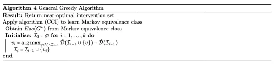
The greedy algorithm relies on the theory developed and the results presented in the appendices of ⁵Ghassami, A., Salehkaleybar, S., Kiyavash, N., & Bareinboim, E. (2018). Budgeted experiment design for causal structure learning. ICML.. This algorithm iteratively adds a variable with the greatest marginal gain to the intervention set, $\Delta_v(\mathcal{I}) = \mathcal{D}(\mathcal{I} \cup \{ v \}) - \mathcal{D}(\mathcal{I}),$ until the budget is exhausted. In other words, it greedily selects a possible intervention. The intractability of computing $\mathcal{D}(\mathcal{I})$ is addressed by proposing a Monte-Carlo approach. The proposed algorithm employs random sampling and generates multisets of DAGs, $G'$, in the algorithm. The following result provides theoretical legitimacy to this method ⁵Ghassami, A., Salehkaleybar, S., Kiyavash, N., & Bareinboim, E. (2018). Budgeted experiment design for causal structure learning. ICML..

Theorem: Imagine we are given some estimate of the number of interventions required to learn the about the edges in the underlying causal graph, with $\mathbb{E}[D(\mathcal{I}, G_i^\prime)] = \mathcal{D}(\mathcal{I})$. If we are given set $\mathcal{I}$ and $\epsilon, \delta > 0$, and if $N = \mid G^\prime\mid > \frac{\mid E(Ess(G^\ast))\mid (2 + \epsilon)}{\epsilon^2}\ln(\frac{2}{\delta}),$ then $\mathcal{D}(\mathcal{I})(1-\epsilon) < \hat{\mathcal{D}}(\mathcal{I}) < \mathcal{D}(\mathcal{I})(1 + \epsilon),$ with probability larger than $1 - \delta.$

Proof: Define $X = \frac{D(\mathcal{I}, G_i^\prime)}{\mid E(Ess(G^\ast))\mid},$ for $i \in \{ 1, \dots, N \}.$ By the assumption of the theorem, $\mathbb{E}[X_i] = \frac{1}{\mid E(Ess(G^\ast))\mid}\mathcal{D}(\mathcal{I}).$ Applying the Chernoff bound we have

$P(\sum_{i=1}^N X_i - \frac{N}{|E(Ess(G^\ast))|} \mathcal{D}(\mathcal{I}) \geq \epsilon \frac{N}{\mid E(Ess(G^\ast))\mid} \mathcal{D}(\mathcal{I}))$

$\leq 2\exp\left(-\frac{N\epsilon^2}{\mid E(Ess(G^\ast)\mid (2 + \epsilon)}\right) \mathcal{D}(\mathcal{I})$

$\leq 2\exp\left(-\frac{N\epsilon^2}{\mid E(Ess(G^\ast)\mid (2 + \epsilon)}\right).$

Therefore,

$P(|\frac{1}{N} \sum_{i=1}^N D(\mathcal{I}, G_i^\prime) - \mathcal{D}(S)|) \geq \epsilon \mathcal{D}(\mathcal{I})$

$\leq 2\exp(-\frac{N\epsilon^2}){\mid E(Ess(G^\ast))\mid (2 + \epsilon)}).$

This further implies

$P(\mid \hat{\mathcal{D}}(\mathcal{I}) - \mathcal{D}(\mathcal{I})\mid$

$< \epsilon \mathcal{D}(\mathcal{I})) > 1 - 2\exp(-\frac{N\epsilon^2}{\mid E(Ess(G^\ast))\mid (2 + \epsilon)}).$

Applying these results, we can set

$N > \frac{\mid E(Ess(G^\ast))\mid (2 + \epsilon)}{\epsilon^2} \ln(\frac{2}{\delta})$

to obtain an upper bound of $1 - \delta$. This completes the proof.

The authors further propose accelerating the greedy algorithm by performing \emph{lazy} evaluations. That is, they exploit the monotonicity of the marginal gains such that if $\Delta_{v_1}(\mathcal{I}_i) > \Delta_{v_2}(\mathcal{I}_i)$ and $\Delta_{v_1}(\mathcal{I}_{i+1}) > \Delta_{v_2}(\mathcal{I}_i)$, then $\Delta_{v_1}(\mathcal{I}_{i+1}) > \Delta_{v_2}(\mathcal{I}_{i+1})$. This improves performance in a similar manner to dynamic programming improvements over naive methods. These procedures are combined to empirically show that a significant portion of causal systems can be learned using only a relatively small number of interventions - a remarkable result for a seemingly intractable problem!

The problem of learning causal structure is still a very active area of research. Extension of work presented here is considered in ⁸Kocaoglu, M., Jaber, A., Shanmugam, K., & Bareinboim, E. (2019). Characterization and learning of causal graphs with latent variables from soft interventions. NeurIPS. and ⁹Jaber, A., & Kocaoglu, M. (2020). Causal discovery from soft interventions with unknown targets: Characterization and learning. for example. For brevity these are not discussed further. We have developed the bulk of the theory necessary to actually implement some useful and promising agents. The next task develops some theory needed to apply some of these tools to the task of imitation learning.

Image credit: Header Image.

References

1. Granger, C. W. J. (1969). Investigating causal relations by econometric models and cross-spectral methods. Econometrica 37:424–438.
2. Spirtes, P., Glymour, C., & Scheines, R. (2000). Causation, Prediction, and Search (2nd ed.). Adaptive Computation and Machine Learning.
3. Kocaoglu, M., Shanmugam, K., & Bareinboim, E. (2017). Experimental design for learning causal graphs with latent variables. NIPS.
4. Bensmail, J., Bonamy, M., & Hocquard, H. (2015). Strong edge coloring sparse graphs. Electronic Notes in Discrete Mathematics 49:773–778.
5. Ghassami, A., Salehkaleybar, S., Kiyavash, N., & Bareinboim, E. (2018). Budgeted experiment design for causal structure learning. ICML.
6. Meek, C. (1995). Causal inference and causal explanation with background knowledge. UAI.
7. Nemhauser, G., Wolsey, L., & Fisher, M. L. (1978). An analysis of approximations for maximizing submodular set functions—I. Mathematical Programming 14:265–294.
8. Kocaoglu, M., Jaber, A., Shanmugam, K., & Bareinboim, E. (2019). Characterization and learning of causal graphs with latent variables from soft interventions. NeurIPS.
9. Jaber, A., & Kocaoglu, M. (2020). Causal discovery from soft interventions with unknown targets: Characterization and learning.

Comments are being migrated. Check back soon.