
In our last discussion we discussed the so-called ‘rung two’ of the ladder of causation, discussing interventions and randomisation in control trials. This is an incredibly important field in the design of experiments. We now take the next step, reaching counterfactual reasoning. Consider for a second how powerful the ability to ask “what if?” really is.
Counterfactuals
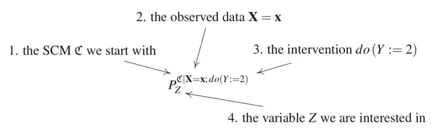
Counterfactuals: Consider some SCM with vertices . We define a counterfactual SCM by replacing the distribution of noise variables: where is an observation and
Peters points out that the new set of noise variables need not be jointly independent. We can thus view counterfactual statements as do-statements in the new (counterfactual) SCM. Further, we can generalise such that only some of the variables of are observed. Consider the counterfactual statement This can be interpreted as asking the question “what would be had we set to 2?”
It is very important to note that different SCMs can be both probabilistically and interventionally equivalent, while still not being _counterfactually equivalent. In fact, Peters presents two different SCMs which generate the same causal graph model while being counterfactually different. This has some important implications:
- Causal graphical models do not present enough information to predict counterfactuals.
- Counterfactual statements require additional assumptions to distinguish between “similar” SCMs which are counterfactually different.
It is also easy to construct an example which proves that counterfactual statements are not transitive. In other words, knowing ” would have been , had been ” and ” would have been , had been ” does not necessarily imply ” would have been , had been .”
An interesting point to consider is counterfactual statements have no correspondence with the real world. Interventional statements, on the other hand, correspond well with randomised controlling of variable - in RCTs for example. The question of whether counterfactual statements are falsifiable are also important to consider, especially in the context of scientific enquiry and judicial procedings for example.
Markov Properties
We are ready to formalise some important statistical properties of causal models.
Markov property: Given a DAG and joint distribution , this distribution is said to satisfy:
- Global Markov property with respect to the DAG if for disjoint sets , where denotes d-seperation and indicates independence.
- Local Markov property with respect to the DAG if each variable is independent of its non-descendants given its parents.
- Markov factorisation property with respect to the DAG if Here are the causal Markov kernels.
These conditions are equivalent given the joint distribution has a density with respect to a product measure.
Markov equivalence of graphs: Let denote the set of Markovian distributions with respect to G: Then two DAGs and are said to be Markov equivalent if This property ensures two graphs entail the same set of independence conditions, as we defined earlier. From this defition the following graphical criteria for the condition has been developed.
Graphical criteria for Markov equivalence: Two DAGs are Markov equivalents if and only if they have the same skeleton and the same immoralities (v-structure).
Markov blanket: Consider DAG and target vertex . The Markov blaket of is the smallest set such that If is Markovian w.r.t. , then
The Markov blanket of Y contains its parents, children and the parents of its children. That is,
SCMs imply Markov property: Assume is induced by an SCM with graph . Then is Markovian w.r.t. .
Next up
This has been a pretty definition heavy discussion, but hopefully it get’s you thinking about the different conditions we need to take into account to formualte a rigorous formulation of causality. Next time we’ll start by discussing causal graphical models and faithfulness.
Resources
This series of articles is largely based on the great work by Jonas Peters, among others:
Image credit: Penguin Image.

Comments are being migrated. Check back soon.