Interventions and Multivariate SCMs

Last time we discussed how we can learn causal structure from data and thought about how this relates to machine learning. Specifically, we noticed that having more data in a semi-supervised learning context can actually lead to descreased performance. Up until this point we have only developed the notions necessary to consider bivariate models - models of no more than two variables. To make this a robust theory we really need to consider models in which there are more than two variables. This raises certain problems. For one, a third variable could be a confounder, a mediator, another parent node, or even another independent effect. We are going to need to consider some additional assumptions necessary to get to a similar method of identifying causal information from data. Developing some graph theory will put us in good stead for later theory, so let’s get straight to it.

Basic Graph Terminology

A graph $G$ consists of vertices $V = \{ 1,\dots,d \}$ and edges $E \subseteq V^2$. We say an edge is undirected if $(i,j)\in E$ and $(j,i)\in E$, otherwise it is directed. If all the vertices of $G$ are directed and $G$ contains no cycles, we say $G$ is a directed acyclic graph (DAG). Three vertices are called a v-structure if one node is a child of two others that are not adjacent. Finally, a permutation $\pi: \\{ 1,\dots,d \\}\rightarrow\\{ 1,\dots,d \\}$ is called a causal ordering if it satisfies $\pi(i) < \pi(j)$ if $j\in DE_i^G$, where $DE_i^G$ are the non-decendants of $i$ in the graph. Any other terminology we need will be developed as we go along. Time for the fun stuff!

Pearl’s d-separation: In a DAG $G$, a path between nodes $i_1$ and $i_m$ is blocked by a set $S$ whenever there is a node $i_k$ such that any of the following holds:

1. $i_k \in S$ and one of the following is true: $i_{k-1} \rightarrow i_k \rightarrow i_{k+1},$ $i_{k-1} \leftarrow i_k \leftarrow i_{k+1}, \quad \text{or}$ $i_{k-1} \leftarrow i_k \rightarrow i_{k+1}$
2. Neither $i_k$ nor any of its descendants is in $S$ and we have that $i_{k-1} \rightarrow i_k \leftarrow i_{k+1}.$

We can extend these conditions to define d-separation for two disjoints sets. We say sets $A$ and $B$ are disjoint if every path between elements the two sets are blocked by another set $S$. We write this formally as $A \perp_G B \mid S.$

Structural Causal Models (Multivariate)

We had previously developed some basic ideas for structural causal models, mostly in the context of 1-3 variables of interest. We now generalise this theory.

Structural Causal Model (SCM): A structural causal model $C = (S, P_N)$ consists of a collection $S$ of $d$ structural assignments. $X_j = f_i(PA_j, N_j),\quad j=1,\dots,d$ where $PA_j$ are the parents of vertex $X_j$; as well as a joint distribution over the noise variables, $P_N = P_{N_1,N_2,\dots,N_d}$.

Proposition: An SCM $C$ defines a unique distribution over the variables $X_1,\dots,X_d$. This is the entailed distribution $P_X^C$, which we may write as $P_X$.

Peters cautions against thinking of these definitions as ‘equations’ because they are, in fact, assignments. We could generate the graph corresponding to an SCM by creating a vertex for each variable, $X_i$ and creating a directed edge from each parent (direct cause) to the variable. We assume this graph is acyclic. Theory dealing with the cyclic assignments has been established, but we don’t consider this further now. An example of generating a set of structural assignments in R is shown below (see Elements of Causal Inference).

# Create some sample from an entailed distribution (taken from EOCI)
set.seed(1)
X3 <- runif(100) - 0.5
X1 <- 2*X3 + rnorm(100)
X2 <- (0.5*X1)^2 + rnorm(100)^2
X3 <- X2 + 2*sin(X3 + rnorm(100))

Interventions

Pearl’s hierarchy - or ladder - of causation places interventional methods as falling on rung two of causal inference. Many of us will be familiar with some of the successes of reinforcement learning. Reinforcement learning, by design, is interventional in its manner of learning, and so it falls squarely in this realm. Eventually we will develop theory to add counterfactual reasoning ability to our reinforcement learning agents, placing it on rung 3 - but let’s not get ahead of ourselves.

The important question for now is how can we model interventional changes in our causal system? Once again, I stess the difference between intervention and conditioning. In general, interventional distributions will differ from conditioned distribtions.

Interventional Distribution: Consider some SCM $C = (S, P_N)$ and its entailed distribution, $P_X$. Assume we replace the assignments for $X_k$ with $X_k = f(\tilde{PA}\_k, \tilde{N}\_k).$ The entailed distribution induced by these new assignments is called the interventional distribution. The variables we changed are said to have been intervened on. We can write this new distribution using do notation by $P_X^C = P_X^{C; do(X_k) = f(\tilde{PA}_k, \tilde{N}_k)}.$

An intervention where the set of direct causes remains unchanged is said to be imperfect. Thinking of our causal model as a graph, the allowed interventions become clear.

Ultimately, we would like to be able to quantify the causal effect of different variables on other variables. This motivates the following definition.

Total Causal Effect (TCE): Given some SCM $C$, there os a total causal effect from $X$ to $Y$ if and only if $X \not\perp Y \quad \text{in } P_X^{C;do(X=\tilde{N}_X)},$ for some random noise variable $\tilde{N}_X.$

Peters develops several equivalent statements for determining whether there is a total causal effect between two variables. Since we will often be thinking about causal models in terms of graphs, I’ll develop the graphical critera for total causal effects.

Graphical Criteria for TCE: Given an SCM with a corresponding graph $G$:

1. If there is no directed path from $X$ to $Y$, then there is total causal effect.
2. It is possible for a directed path to exist without any total causal effect.

One of the biggest achievements in the design of experiments was popularised by Fisher in The Design of Experiments in which he develops the randomised control trial (RCT). This process of randomisation of a certain variable removes any causal links by intervening on it. This was pivotal to biochemical industry in which placebo effects are crucial to quantify.

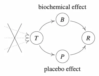
In studies of new drugs, we would like to be able to distinguish the effects of the drug from placebo. Consider two treatments, $T=1$and $T = 2$, while $T= 0$ represents no treatment. By randomising on treatment, we remove possible confounding causes on treatment. Assuming the placebo effect is the same for both the drug and the no drug situations, we have structural assignments that satisify:

$f_P(T=0, N_P) \neq f_P(T=1, N_P) = f_P(T=0, N_P).$

Voila! Observing a dependence of recovery on treatment now establishes a causal link (under the causal model assumptions).

Next Up

Nex time we step up a rung on the ladder of causation, finally reaching counterfactual reasoning - a tremendous contribution of the field of causal inference.

Resources

This series of articles is largely based on the great work by Jonas Peters, among others:

• Elements of Causal Inference
• The Book of Why
• Jonas Peters Lecture Series

Comments are being migrated. Check back soon.