Causality and Machine Learning

Last time we briefly discussed the theory needed to start thinking about how we can learn, in the statistical sense, causal information from ‘dumb’ data. Some key points were that identifiability of a causal model is a crucial aspect of the analysis. Whether or not the model is identifiable is, in large part, dependent on the nature of the noise. We discussed the results under the assumption of linear non-Gaussian noise, among other cases. I also proceeded to tease the ‘machine learning’ aspect - we’re almost there, I promise!

This Series

A Causal Perspective
Causal Models
Learning Causal Models
Causality and Machine Learning
Interventions and Multivariate SCMs
Reaching Rung 3: Counterfactual Reasoning
Faithfulness
The Do Calculus

Structure Identification

We have formulated causal relationships as directed acyclic graphs (DAGs) up to this point. The problem we now face is how to apply the identifiability results from previous discussions to identifying and building causal structural models for the data. This is a very challenging learning problem and the results we now discuss are very much current research and bound to change.

Additive Noise Models

Once again we can look at the simple case of additive noise models. The first method tests the independence of the residuals in the data. This is a special case of the RESIT algorithm we shall discuss in the future. This algorithm runs as follows:

Regress \( Y \) on \( X \) such that we can write \( Y \) as a function of \( X \) and a noise term.
Test the independence between \( Y - \hat{f}_Y(X) \) and \( X \).
Repeat steps (1) and (2), switching the roles of \( X \) and \( Y \).
If one direction is independent but the other isn’t, infer the former direction as causal.

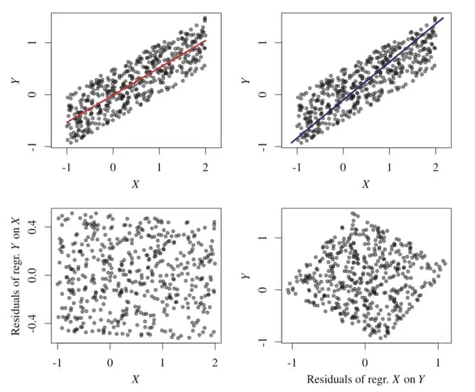
Peter’s provides an informative example of this testing procedure in action using a simple example. The left side corresponds to the \( X \) data while the right displys the \( Y \) data. Regression procedures are shown in the top row with corresponding residuals shown below. It is clear that there is a dependence for the \( X \) on \( Y \) direction. Applying the algorithms above, we infer a causal direction, \( X \rightarrow Y \).

An alternative approach is to apply a maximum likelihood method. We compare the causal directions by comparing the associated likelihood scores. These are computed as \[ L_{X\rightarrow Y} = -\log \hat{var}[X] -\log \hat{var}[R_Y], \] where \( R_Y \) are the residuals. We repeat this for the \( Y \rightarrow X \) direction. An R code example, modified from Elements of Causal Inference, is shown below.

library(dHISC) # For 'dhsic.test' independence test
library(mgcv) # For 'gam' nonlinear regression method

set.seed(1)
X <- rnorm(500)
Y <- X^3 + rnorm(500)

forward.model <- gam(Y ~ s(X))
backward.model <- gam(X ~ s(Y))

dhsic.test(forward.model$residuals, X)$p.value # [1] 1
dhsic.test(backward.model$residuals, Y)$p.value # [1] 0.000999001

# Compute likelihoods
-log(var(X)) -log(var(forward.model$residuals)) # [1] -0.1265013
-log(var(backward.model$residuals)) -log(var(Y)) # [1] -1.682779

Semi-Supervised Learning

Suppose we are given some training data with labels in the form \( (D_1,A_1),\dots,(D_n,A_n) \) where each of the \( D_i \) is a dataset such that \[ D_i = { (X_1,Y_1),\dots,(X_n,Y_n) } \] containing i.i.d. realisations from the distributition \( P_{X,Y}^i \). The label \( A_i \in \{ \rightarrow,\leftarrow \} \) such that it describes the causal direction between the pair \( (X,Y). \) Since we now have labled training data, this learning problem becomes a supervised statistical learning prediction problem.

In supervised learning scenarios we are given a sample of labled data points drawn from some joint distribution. Formally, \[ (X_1,Y_1),\dots,(X_n,Y_n) \sim^{\text{i.i.d.}} P_{X,Y}. \] This gives us information about the conditional distribution \( P_{X\|Y} \) which we can exploit. In semi-supervised learning we are given an additional \( m \) unlabled data points. Since these points are not conditioned, one would hope this would give information about the unconditional distribution, \( P_X \).

In previous discussions we developed notions for talking about causal structure of two variables. In this case, a variable is either causal or anitcausal. Tradtionally, machine learning engineers do not consider the underlying causal structure. This is a danger.

Contrary to popular belief, more data does not always solve our issues - in fact, it can make it worse!

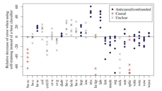
Recall, we discussed that causal conditional distributions are independent of each other. This necessarily means the distribution of the one does not contain information about the distribution of the other. The following figure nicely demonstrates the performance of self-supervised learning agents on different datasets. We immediately notice that when causal data is used to predict an effect, additional data hurts performance when comparing against some base classifier. This is remarkable, but intuitive.

Next up

Up until this point we have only developed the theory in the context of bivariate distrubutions - the case for two variables. Next time we’ll start developing the theory for the multivariate, more general case. We’ll introduce some basic graph theory and develop some important definitions and results for later interesting application.

Resources

This series of articles is largely based on the great work by Jonas Peters, among others: