 St John
In the last episode we developed the first tools we need to develop the theory needed to formalise interventions and counterfactual reasoning. In this article we’ll discuss how we can go about learning such a causal model from some observational data, and what constraints are required for doing this. Note, this is an active area of research and so we really don’t have all the tools yet. This should be both a cautionary note and an exciting motivation to get involved in this research! This is really when the theory of causal inference starts to get exciting, so tighten your seat-belts.
This Series
- A Causal Perspective
- Causal Models
- Learning Causal Models
- Causality and Machine Learning
- Interventions and Multivariate SCMs
- Reaching Rung 3: Counterfactual Reasoning
- Faithfulness
- The Do Calculus
Identifiability
Previously, we discussed the idea that an SCM induces a joint distribution over the variables of interest. For example, the SCM \( C \rightarrow E \) induces \( P_{C,E} \). Naturally, we wonder whether we can identify, in general, whether the joint distribution came from the SCM \( C \rightarrow E \) or \( E \rightarrow C \). It turns out, the graphs are not unique. In other words, structure is not identifiable from the joint distribution. Another way of phrasing this is the graph adds an additional layer of knowledge.
Non-uniqueness of graph structures: For every joint distribution \( P_{X,Y} \) of two real-valued variables, there is an SCM \[ Y = f_Y(X,N_Y), X \perp Y, \] where \( f_Y \) is a measurable function and \( N_Y \) is a real-valued noise variable.
This proposition indicates that we can construct an SCM from a joint distribution in any direction. This is crucial to keep in mind, especially if we plan on trying to use observational data to infer causal structure.
We are now ready to discuss some methods of identifying cause and effect with some a priori restrictions on the class of models we are using.
Additive Noise Models
Our first class of model are the linear non-Gaussian acyclic models (LiNGAMs). Here we assume that the effect is a linear function of the cause up to some additive noise term, \[ E = \alpha C + N_E, \quad \alpha\in\mathbb{R} \] Note, we are explicitly removing the possibility that the additive noise is Gaussian in nature. With this restrictive assumption in place, we can formulate the identifiability result we are looking for:
Identifiability of linear non-Gaussian models: Given the joint distribution \( P_{X,Y} \) having linear model \[ Y = \alpha X + N_Y, \quad N_Y \perp X, \] with continuous random variables \( X, N_Y, Y \), there exists \( \beta\in\mathbb{R} \) and random variable \( N_X \) such that \[ X = \beta Y + N_X, \quad N_X \perp Y, \] if and only if \( N_Y \) and \( X \) are Gaussian.
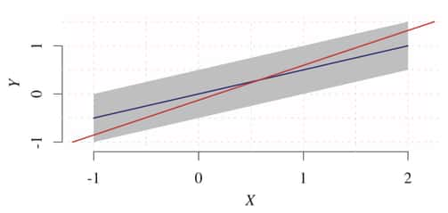
Peters provides a lucid example of this in action. Here we have uniform noise over \( X \) and a linear relationship between the variables of interest. The backwards model, shown in blue, is not valid because the noise term over \( X \) is not independent of the variable \( Y \), violating the independence condition.
Interestingly enough, non-Gaussian additive noise can be applied to estimating the arrow of time from data!
We are now ready to extend the discussion the nonlinear additive noise models.
Additive noise model (ANM): The joint distribution \( P_{X,Y} \) is said to admit an ANM from \( X \) to \( Y \) if there is a measurable function \( f_Y \) and a noise variable \( N_Y \) such that \[ Y = F_Y(X) + N_Y, \quad N_Y \perp X. \]
We can extend the identifiability condition to include ANMs as well. For brevity I shall not include it. Peters, however, provides a nice description and proof sketch in chapter 4 of his book. Further extensions, such as to discrete ANMs and post-nonlinear models, are possible and described in the literature.
Information-Geometric Causal Inference
We now turn to the idea of formalising the independence condition between \( P_{E|C} \) and \( P_C \). Assuming the (strong) condition that \[ Y = f(X) \quad\text{and}\quad X = f^{-1}(Y),\] the principle of independence of cause and mechanism simplifies to the independence between \( P_X \) and \( f \).
Avoiding the detailed mathematics for now, the results show that the uncorrelatedness of \( \log(f’) \) and \( p_X \) necessarily implies correlation between \( \log(f^{-1’}) \) and \( p_Y \). The logarithms here are used for the sake of interpretibility of the result, but it is not a necessary formulation for the result to hold.
It has been shown, as we shall soon come across, that the performance of semi-supervised learning methods is dependent on the causal direction. IGCI can explain this using assumptions similar to what we have just discussed.
Next up
With that reference to machine learning, that should satisfy for curiosity - at least temporarily. In the next session we’ll take this idea further and discuss some more theory before jumping into the problem of machine learning.
Resources
This series of articles is largely based on the great work by Jonas Peters, among others:
