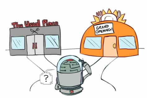
The active inference framework proposes agents act to maximise the evidence for a biased generative model, whereas in reinforcement learning the agent seeks to maximise the expected discounted cumulative reward. In Reinforcement Learning Through Active Inference a new RL objective - the free energy of the expected future - is implemented by augmenting traditional learning techniques with concepts from active inference theory. This approach has two important side effects.
- A balance between exploration and exploitation is intrinsic.
- It allows for a sparsity and lack of reward.
Both RL and active inference highlight the importance of probabilistic models, planning efficiently, and inferring explicitly about the environment. In the context of active inference, agents seek to maximise their Bayesian model evidence for their generative model \( p^\Phi(o,s,\theta) \), where \( \theta \) are model parameters. This generative model can be biased towards observations that are likely and beneficial for an agent’s success. Rewards are treated as prior probabilities over some observation, \( o \). The divergence, \( D_{KL} \), between the preferred and the expected outcome is used as a measure of the success of this model.
Free Energy theory tells us that agents can perform approximate Bayesian inference by minimising the variational free energy. Given some distribution \( q(s,\theta) \), and some generative model \( p^\Phi(o,s,\theta) \), the free energy is given by \[ F = D_{KL}[q(s,\theta)||p^\Phi(o,s,\theta)]. \] In this formulation, we treat the model parameters \( \theta \) as random variables. We are thus treating the learning process as a process of approximate inference. In this formulation, agents maintain beliefs about about policies \( \pi = {o_0,\dots,o_T} \). Policy selection can thus be formulated as a process of approximate inference over the distribution of policies, \( q(\pi) \).
Since a policy holds information about a sequence of variables in time, the free energy formulation needs to be altered so as to incorporate future variables. This leads directly to the formulation of the free energy of the expected future - a quantity we wish to minimise, defined as \[ \tilde{F} = D_{KL} [q(o_{0:T},s_{0:T},\theta,\pi) || p^\Phi(o_{0:T},s_{0:T},\theta)], \] where \( q(o_{0:T},s_{0:T},\theta,\pi) \) is the agent’s belief about future variables, and \( p^\Phi(o_{0:T},s_{0:T},\theta) \) is the generative model. \[ \tilde{F} = 0 \implies D_{KL} [q(\pi) ||-e^{-\tilde{F}_{\pi}}] = 0 \] where \[ \tilde{F}_{\pi} = D_{KL}[q(o_{0:T},s_{0:T},\theta|\pi) || p^\Phi(o_{0:T},s_{0:T},\theta)]. \] This gives the result that the free energy of the expected future is minimised when \( q(\pi) = \sigma(-\tilde{F}_\pi) \). Therefore, policies that minimise \( \tilde{F}_\pi \) are more likely.
Naturally, the question arises as to what minimising this quantity, \( \tilde{F}_\pi \), means. Assuming the model is only biased in its beliefs of observations, the authors propose factorising the agent’s generative model as follows: \[ p^\Phi(0_{0:T},s_{0:t},\theta) = p(s_{0:t},\theta|0_{0:T})p^\Phi(0_{0:T}). \] Here, \( p^\Phi(0_{0:T}) \) is a distribution over preferred rewards - since this is the goal in RL. Using this factorisation, it can be shown that \( \tilde{F}_\pi \) can be broken down into two terms representing distinct concept, \[ -\tilde{F}_\pi \simeq -E_{q(0_{0:T}|\pi)}[D_{KL}[q(s_{0:T},\theta|o_{0:T},\pi) || q(s_{0:T},\theta|\pi)]] + E_{q(s_{0:T,\theta|\pi})}[D_{KL}[q(o_{0:T|s_{0:T},\theta,\pi}) || ^\Phi(o_{0:t})]].\]
The expected information gain is crucial as it quantifies the amount of information an agent believes it will gain by following some policy. This term promotes exploration of the state and parameter spaces, since agents hold beliefs about both the state of the environment and its own model parameters.
The minimisation of the extrinsic term is, by definition, the minimisation of the difference between what the agent believes about future observations and what it would prefer to observe. In other words, it measures how much reward it expects to see in the future in contrast to how much reward it would like to achieve. This is exploitation. This result is key as a natural balance between exploration and exploitation is a fundamental issue in reinforcement learning in general.
This objective is evaluated in three steps:
- Evaluate beliefs,
- Evaluate \( \tilde{F}_\pi \), and
- Optimise \( q(\pi) \) such that \( q(\pi) = \sigma(-\tilde{F}_\pi) \)
 St John
