So Many Options!

Introduction

Fokker-Planck equations, and stochastic differential equations in general, have many powerful applications in a wide ranging set of fields. These include modelling of Brownian motion in physical systems, electronic noise in engineering fields, and behaviour of financial assets in quantitative finance.

This paper looks at the specific application of the Fokker-Planck equation to modelling valuation of stock options using the Black-Scholes equation. From this equation, one can derive the Black-Scholes formula, giving an estimate of the value of a European option.

This formula laid the mathematical foundation for options trading, providing much needed legitimacy to the trade of stock options. In fact, the formula was so instrumental in the development of options trading that Myron Scholes and Robert Merton were awarded the Nobel Prize in Economics in 1997 for related work. Fischer Black was not awarded the prize as it is not awarded posthumously. First some relevant financial theory will be explored. The appropriate mathematics will be developed and briefly discussed before applying it to the financial mathematics explored in this paper. Finally, some simulations will be presented with accompanying Python code.

Financial Theory

Options

A stock option is a financial contract in which the holder of the option is granted the right to buy or sell some financial asset at a specified price. An option that may be exercised before or on expiration is known as an American option, while an option that may only be exercised on the date of expiry is called a European option. The incentive for owning stock options is that it changes the risk profcile of a trade in contrast to conventional buying or selling of stocks. An option can be thought of as a way to increase or decrease trading risk by increasing or decreasing the potential payout. This basic principle allows for different trading strategies by betting on the expected future behaviour of an underlying asset. For example, one can use an option as an insurance policy on the purchase of an underlying stock.

Valuation

The valuation (pricing) of an option is a non-trivial task. The value depends on both the value of the underlying financial object (asset) and a number of variables associated with the risk and potential payout of the option. In general, the following variables are used to calculate the price of an option:

Market price of underlying asset.
The strike price of the option.
Cost of holding underlying asset.
Time to expiration.
Estimate of volatility of underlying asset.

This paper focuses on the application of a Fokker-Planck equation - in the form of the Black-Scholes equation - for option valuation.

Wiener Processes & Brownian Motion

The Wiener process is a real-valued continuous-time stochastic process. It forms an important aspect of theories in many fields, including mathematics, economics, biology and physics. It is often referred to as Brownian motion because of the strong ties with the physical theory of random particle motion. It is a well-known example of a Lévy process - a continuous-time random walk. A Wiener process $W_t$ is characterised as in Essentials of Stochastic Processes [1].

$W_0= 0$.
$W$ has independent increments: for every $t>0$, the future increments $W_{t+u} - W_t,$ $u \ge 0$, are independent of the past values $W_s$, $s\leq t.$
$W$ has Gaussian increments: $W_{t+u} - W_t$ is normally distributed with mean $0$ and variance $u$, $W_{t+u} - W_t\sim \mathcal N(0,u).$
$W$ has continuous paths: $W_t$ is continuous in $t$.

Geometric Brownian Motion

Geometric Brownian motion is a continuous-time stochastic process where the logarithm of the stochastic quantity follows a Wiener process. A stochastic process $S_t$ is said to follow a GBM if it satisfies the stochastic differential equation $dS_t = \mu S_t dt + \sigma S_t dW_t,$ where $W_t$ is a Wiener process, $\mu$ is the drift, and $\sigma$ is the volatility. It is particularly well-known for its use in mathematical finance to model stock prices. This paper explicitly focuses on the Black-Scholes model - an example of geometric Brownian motion satisfying a stochastic differential equation.

Itô calculus

Itô calculus extends the mathematical formulation of calculus to stochastic processes. This is especially relevant for options pricing as the Black-Scholes equation is a stochastic differential equation which employs Itô calculus to solve for the Black-Scholes formula. The central concept in this formulation is a generalisation of the Riemann-Stieltjes integral. We define the integral of some process $H_s$ as $Y_t = \int_0^t H_sdX_s,$ where X is a Wiener process. The integral is defined as the limit of a sequence of random variables, which gives another stochastic process. A key result in Itô calculus is as follows.

Definition: For an Itô drift-diffusion process $dX_t = \mu_tdt + \sigma_tdB_t$ and any twice differentiable function $f(t,x)$ of two real variables $t$ and $x$, we have $df(t,X_t) = (\frac{\partial f}{\partial t} + \mu_t\frac{\partial f}{\partial x} + \frac{1}{2}\sigma_t^2\frac{\partial^2 f}{\partial x^2})dt + \sigma_t\frac{\partial f}{\partial x}dB_t.$

Fokker-Planck Equations

The Fokker-Planck equation, in the context of statistical mechanics, is a partial differential equation used to model the time evolution of some probability density of particle velocities subject to drag and stochastic forces. The equation can be generalised for application to different systems. This paper will focus on the application to financial modelling of European option pricing.

An interesting result, which ties together the mathematical formulations of various fields, is that every Fokker-Planck equation is equivalent to some path integral. Consider, for example, Feynman’s path integral formulation of quantum mechanics. This theorem tells us that we can formulate quantum mechanics in terms of Fokker-Planck equations. Alternatively, the non-equilibrium statistical mechanics formulation, for which the Fokker-Planck equation was developed, can be written in terms of path integrals. Given some Wiener process $W_t$ described by $dX_t = \mu(X_t,t)dt + \sigma(X_t,t)dW_t$, with $\mu(X_t,t)$ being the drift, we can describe the Fokker-Planck equation for density $p(x,t)$ of random variable $X_t$ as

\[\frac{\partial}{\partial t}p(x,t) = -\frac{\partial}{\partial x}[\mu (x,t)p(x,t)] + \frac{\partial^2}{\partial x^2}[D(x,t)p(x,t)].\]

This generalises easily to higher dimensions.

Asset Pricing Applications

Stock assets are often modelled as following a geometric Brownian motion. The Black-Scholes dynamic is given by $\frac{dS_t}{S_t} = \mu dt + \sigma dB_t.$ Applying Itô lemma to $f(x)=\ln(x)$, we can solve this stochastic differential equation [2]. $f'(x)=\frac{1}{x}$ $f''(x)=-\frac{1}{x^2}$

\[d(ln(X_t)) = \frac{1}{X_t} dX_t -\frac{1}{2X_t^2} d<X_t>\\ = \mu dt + \sigma dW_t - \frac{\sigma^2}{2} dt\\ = \mu dt + \sigma dW_t - \frac{\sigma^2}{2} dt\\ = (\mu - \frac{\sigma^2}{2}) dt + \sigma dW_t\]

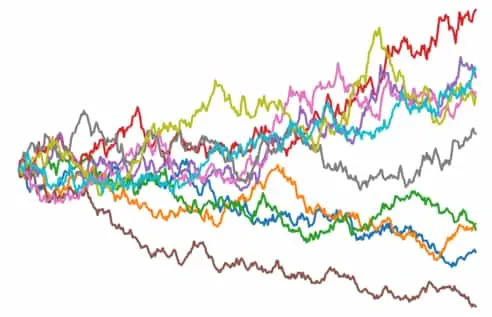
Which gives the result, $ln(X_t)-ln(X_0)=ln(\frac{X_t}{X_0})=(\mu - \frac{\sigma^2}{2})(t-0) + \sigma W_t$ $X_t=X_0 e^{(\mu - \frac{\sigma^2}{2})t + \sigma W_t}$

$S_T = S_0e^{(\mu-\frac{\sigma^2}{2})T+\sigma B_T}.$ This form of the equation can be used to simulate price movements of an asset.

The Black-Scholes Equation

The Black-Scholes equation is insightful as it enforces that one can perfectly hedge the financial option by trading the underlying financial asset - essentially eliminating risk. Moreover, there is only one correct value for the option. This value is given by the formula.

\[\frac{\partial V}{\partial t} + \frac{1}{2}\sigma^2S^2\frac{\partial^2V}{\partial S^2} + rS\frac{\partial V}{\partial S} - rV = 0\]

Black-Scholes Derivation

This derivation is based on Ten Different Ways to Derive Black–Scholes[3]. This derivation involves Fokker-Planck Equations. First, assume the option value is determined by the present value of the risk-neutral expected payoff. Also consider $p(S^*,t^*;S,T)$ to be the transition probability density for the risk-neutral random walk where $S^\ast$ is the current asset price and $t^*$ is the current date. $K$ is the strike price and $T$ is the expiration date. Then, the value of the stock option is $V(K,T)$ where,

\[V(K,T) = e^{-r(T-t)}E_t[max(S_T-K,0)] \\ = e^{-r(T-t^*)}\int_0^\infty max(S-K,0)p(S^*,t^*;S,T)ds \\ = e^{-r(T-t^*)}\int_0^\infty (S-K)p(S^*,t^*;S,T)ds\]

Differentiating with respect to $K$, the strike price, we get

\[\frac{\partial V}{\partial K} = e^{-r(T-t^*)}\int_K^\infty p(S^*,t^*;S,T)ds \\ \frac{\partial^2 V}{\partial K^2} = e^{-r(T-t^*)} p(S^*,t^*;S,T)\]

This gives the transition density in a tractable form,

\[p(S^*,t^*;S,T) = e^{r(T-t^*)} \frac{\partial^2 V}{\partial K^2}.\]

Since this is a density, we can apply the Fokker-Planck equation to get an equation for the time evolution of this density.

\[\frac{\partial p}{\partial T} = \frac{1}{2} \frac{\partial^2}{\partial S^2}(\sigma^2S^2p) - \frac{\partial}{\partial S}(rSp)\]

Now, instead considering the change in value with respect to the expiration date, $T,$ subbing in for $\frac{\partial p}{\partial T}$, and integrating by parts we get

\[\frac{\partial V}{\partial T} = -rV + e^{-r(T-t^*)} \int_K^\infty (S-K) \frac{\partial p}{\partial T} dS \\ = -rV + e^{-r(T-t^*)} \int_K^\infty (S-K) [\frac{1}{2} \frac{\partial^2}{\partial S^2}(\sigma^2S^2p) - \frac{\partial}{\partial S}(rSp)] dS \\ = -rV + \frac{1}{2}e^{-r(T-t^*)}\sigma^2K^2p + re^{-r(T-t^*)}\int_K^\infty SpdS\]

Finally, we get the form of the Black-Scholes equation,

\[\frac{\partial V}{\partial T} = \frac{1}{2}\sigma^2K^2 \frac{\partial^2 V}{\partial K^2} - rK\frac{\partial V}{\partial K}\]

The Traditional Derivation

This derivation is based on Options, Futures and Other Derivatives [4]. This argument is similar to that orginally made by Black and Scholes in their original paper. We start by assuming the underlying asset takes the form and behaves like a geometric Brownian motion. $\frac{dS}{S} = \mu dt + \sigma dW,$ where W is some Wiener process. $W$ is the only source of randomness in this equation. We thus have $E[\frac{dS}{S}] = \mu dt$, with variance $\sigma^2dt.$ Since we know the value at expiry of some European option is given by $V(S,T)$, we can apply Itô’s lemma for two variables to get,

\[dV = \left(\mu S \frac{\partial V}{\partial S} + \frac{\partial V}{\partial t} + \frac{1}{2}\sigma^2 S^2 \frac{\partial^2 V}{\partial S^2}\right)dt + \sigma S \frac{\partial V}{\partial S}\,dW.\]

Now consider a delta-neutral portfolio with value $\Pi = -V + \frac{\partial V}{\partial S}$. Over some $\Delta t$, the total change in value is $\Delta\Pi = -\Delta V + \frac{\partial V}{\partial S}\Delta S$. Discretising and substituting in for $\Delta V$ and $\Delta S$, we get

\[\Delta \Pi = \left(-\frac{\partial V}{\partial t} - \frac{1}{2}\sigma^2 S^2 \frac{\partial^2 V}{\partial S^2}\right)\Delta t.\]

Notice now that the term involving $W$ is no longer part of the equation. Effectively, this portfolio is now riskless. This portfolio must have a rate of return equal to that of the risk-free rate of return, otherwise there would exist oppurtunities for riskless arbitrage. So we have $r\Pi\Delta t = \Delta\Pi$. We can then equate for $\Delta\Pi$.

\[\left(-\frac{\partial V}{\partial t} - \frac{1}{2}\sigma^2 S^2 \frac{\partial^2 V}{\partial S^2}\right)\Delta t = r\left(-V + S\frac{\partial V}{\partial S}\right)\Delta t\]

Simplyfying, we arrive at the result of the Black-Scholes PDE:

\[\frac{\partial V}{\partial t} + \frac{1}{2}\sigma^2 S^2 \frac{\partial^2 V}{\partial S^2} + rS\frac{\partial V}{\partial S} - rV = 0\]

The Black-Scholes Formula

Imposing boundary conditions on the Black-Scholes Equation allows us to obtain a formula for the price of European options. This is the famous equation Black and Scholes revealed in their seminal work. The following boundary conditions are relevant for the Black-Scholes PDE derived in previous sections. We can solve this PDE as in [4] by applying these conditions and using methods of Itô calculus.

$C(0,t)$ = 0 for all t
$C(S,t) \longrightarrow S$ as $S \longrightarrow \infty$
$C(S,T) = \max {S-K,0}$

Condition 3 above gives the value of the option at the time of expiry, T. There are other boundary conditions available when considering different limits, but these give the same resulting equation as we should expect for consistency. Let us observe that the SDE is a Cauchy-Euler equation. We can introduce some change of variables to form it as a diffusion equation. Consider,

$\tau = T-t,$
$Ce^{r\tau},$ and
$x = \ln{S/K} + (r-\frac{1}{2}\sigma^2)\tau,$

which yields the diffusion equation $\frac{\partial u}{\partial \tau} = \frac{1}{2}\sigma^2\frac{\partial^2u}{\partial x^2}.$ Condition 3 becomes an initial condition $u(x,0) = u_0(x) = K(\exp{\max{x,0}}-1).$ Applying this initial condition, we can solve the diffusion equation using convolution methods.

\[u(x,\tau) = \frac{1}{\sigma \sqrt{2\pi\tau}}\int_{-\infty}^\infty u_0(y)e^{-\frac{(x-y)^2}{2\sigma^2\tau}}dy \\ = Ke^{x+\frac{1}{2}\sigma^2\tau}N(d_1)-KN(d_2).\]

Here $d_1$ and $d_2$ are

\[d_1 = \frac{1}{\sigma\sqrt{\tau}}[(x+\frac{1}{2}\sigma^2\tau)+\frac{1}{2}\sigma^2\tau] \\ d_2 = \frac{1}{\sigma\sqrt{\tau}}[(x+\frac{1}{2}\sigma^2\tau)-\frac{1}{2}\sigma^2\tau].\]

This is (without proof) equivalent to the traditional formulation. For a non-dividend-paying underlying asset,

\[C(S_t, t) = N(d_1)S_t - N(d_2) PV(K) \\ d_1 = \frac{1}{\sigma\sqrt{T - t}}\left[\ln\left(\frac{S_t}{K}\right) + \left(r + \frac{\sigma^2}{2}\right)(T - t)\right] \\ d_2 = d_1 - \sigma\sqrt{T - t} \\ PV(K) = Ke^{-r(T - t)}\]

$N(\cdot)$ is the cumulative normal distribution (CDF of a normal).
$T-t$ is the time to expiry.
$S_t$ is the stock price (spot price).
$K$ is the strike price of the option.
$r$ is the risk free rate.
$\sigma$ is the volatility of the asset.

The Black-Scholes formula, $C(S_t,t)$, gives the price for a European style call option. There are two terms in this equation. The first term, $N(d_1)S_t$, is given with the stock price at present value. $K$ is the strike price, which is not a present value. We therefore discount the strike price by subtracting off the time-value of money. That is, we remove the interest one would get with a risk-free investment - think government bond. We then get $PV(K) = Ke^{-r(T - t)}.$ The key here is that we assume the periodic daily returns are normally distributed [6]. Integrating over this normal distribution on the interval $[a,b]$ gives the probability of observing a return in that interval. $N(d_1$ is the expected value of the stock, multiplied by the probability that the stock price will reach or exceed the strike price. $N(d_2)$ is the probability that the stock price will be equal to or greater than the strike price when the stock option reaches the date of expiry.

Dangers & Pitfalls

The Black-Scholes model provided much needed mathematical rigour and legitimacy to options trading, however emphasis is placed on the fact that this is a model. The aphormism “all models are wrong, but some are useful” is especially relevant here since we are dealing with financial assets. Most of the issues with the model arise directly from the assumptions that are made about the market itself. The following limitations of the Black-Scholes model [6] should be carefully considered before applying the techniques discussed in this paper.

Tail risk - Underestimation of extreme movements in stock prices. The assumption of normally distributed stock prices is criticised as extreme price movements have been shown to occur far more often than predicted by a normal distribution.
Liquidity risk - The assumption of instant and cost-less trading.
Volatility risk - The assumption of stationarity. Critics argue that large fluctuations in price cannot be ignored.
Gap risk - Assumption of continuous time and trading.
Independence - The assumption that price movements at subsequent time steps are independent of previous time steps is flawed. Studies of assets has shown short-term and long-term dependence.

Code

    from scipy.stats import norm

    def d1(sigma, time_to_expire, S, K, r):
        return (math.log(S/K) + (r + sigma**2 / 2) * (time_to_expire)) 
            / (sigma * math.sqrt(time_to_expire))

    def d2(sigma, time_to_expire, S, K, r):
        return d1(sigma, time_to_expire, S, K, r) - sigma * math.sqrt(time_to_expire)

    def PV(K, r, time_to_expire):
        return K * math.exp(-r*(time_to_expire))

    def black_scholes(sigma, time_to_expire, S, K, r):
        return norm.cdf(d1(sigma, time_to_expire, S, K, r)) * S 
        - norm.cdf(d2(sigma, time_to_expire, S, K, r)) * PV(K, r, time_to_expire)

    # Plot option value as a function of multiple variables
    from mpl_toolkits import mplot3d
    fig = plt.figure()
    ax = plt.axes(projection='3d')

    S = np.linspace(0.01,2,50)
    T = np.linspace(0,2,101)

    X, Y = np.meshgrid(S, T)
    Z = np.zeros((len(S),len(T)))

    for i in range(len(S)):
        for j in range(len(T)):
            Z[i,j] = black_scholes(volatility, T[j], S[i], 1, 0.02)

    scamap = plt.cm.ScalarMappable(cmap='inferno')
    fcolors = scamap.to_rgba(X)

    ax.view_init(45, -80)
    ax.plot_surface(X,Y,np.transpose(Z), facecolors=fcolors)
    ax.set_xlabel("S")
    ax.set_ylabel("T")
    ax.set_zlabel("Option Value")
    ax.set_title("Option value as a function of\ntime to expiry (T) and asset price (S)")

    fig.savefig("3DOptionPrices.png", dpi=400)

[1] Essentials of Stochastic Processes. Springer, 1996.
[2] SRKX (https://quant.stackexchange.com/users/467/srkx). What is ito’s lemma used for in quantitativefinance? Quant Stack Exchange.
[3] Newsmth.net. Ten different ways to derive black–scholes, 2020.
[4] John C. Hull.Options, Futures and Other Derivatives. Pentice Hall, 2008.
[5] Black scholes: A simple explanation - youtube.
[6] Jørgen Veisdal. The black-scholes formula, explained.https://medium.com/cantors-paradise/the-black-scholes-formula-explained-9e05b7865d8a. Accessed: 5-04-2020

References

- Durrett, R. (1996). Essentials of Stochastic Processes. Springer.
- SRKX What is Itô's lemma used for in quantitative finance?. Quantitative Finance Stack Exchange.
- Newsmth.net (2020). Ten different ways to derive Black–Scholes.
- Hull, J. C. (2008). Options, Futures and Other Derivatives. Prentice Hall.
- Veisdal, J. (2020). The Black-Scholes formula, explained. Cantor's Paradise (Medium).
Comments are being migrated. Check back soon.