The Mathematics of Predictive Processing

Hello! Today we’ll be discussing the mathematics of predictive processing - a modern theory for how much of the processing of information is done in the brain. This is also an active area of research with an impact on research in many fields including reinforcement learning. Feel free to follow along with the video presentation embedded below.

Introduction

1. Predictive Coding
2. Perception
3. Let’s use some mathematics (since we’re in this dept)
4. Let’s approximate
5. Neural implementation
6. Hebbian learning
7. Free Energy
8. Discussion

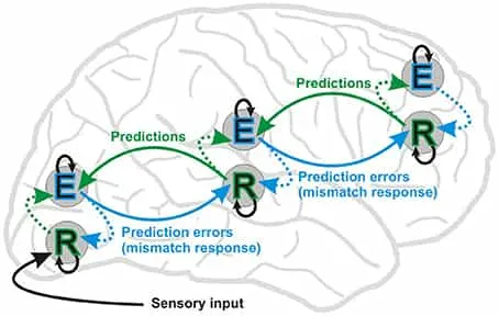
All neural processes consists of two streams: bottom-up stream of sense data, and a top-down stream of predictions. Minimize surprise/free energy- the error between prediction and sense data… To produce/update an effective (but `simple’!) model of our world.

Biological Constraints:

1. Local computation - neuron only performs computation on the basis of activity of inputs and associated weights
2. Local plasticity - synaptic plasticity only based on activity of pre-synaptic and post-synaptic neurons

A motivated example

Let’s talk through an example. Consider the problem of inferring the value of a single variable from a single observation. For example, a simple organism trying to estimate food size from observed light intensity.

1. Let $v$ be the food size
2. Let $g$ be a non-linear function relating size to light intensity
3. Then $u$ is a noisy estimate of the light intensity s.t. $u \sim N(g(v),\Sigma_u)$

How could our animal ‘compute’ the expected food size explicitly? $p(v|u) = \frac{p(v)p(u|v)}{p(u)}$ $p(u) = \int p(v)p(u|v)$ Why is this a problem?

Posterior distribution might not take a ‘standard’ form - we would not be able to use basic summary statistics to describe the distribution. How would we compute that integral? Nontrivial. And so comes the physicists best friend - approximation!

The approximate solution!

We now find the most likely size, denoted $\phi$, that maximises $p(v|u)$ instead of finding the whole posterior distribution. The posterior density is thus $p(\phi |u)$. Here $p(\phi|u) = \frac{p(\phi)p(u|\phi)}{p(u)}$ but $p(u)$ does not depend on $\phi$ We want to find $\phi$ to maximise the posterior. We do this by maximising $F = \ln(p(\phi)p(u|\phi)) = \ln(p(\phi)) + \ln(p(u|\phi))$ $F = \frac{1}{2} ( -\ln(\Sigma_p) - \frac{(\phi-v_p)^2}{\Sigma_p} -\ln(\Sigma_u) -\frac{(u-g(\phi))^2}{\Sigma_u}) + C$ Update $\phi$ proportionally to $\frac{\partial F}{\partial \phi} = \frac{v_p-\phi}{\Sigma_p} + \frac{u - g(\phi)}{\Sigma_u}g'(\phi)$

Neural implementation and learning

Notice $\epsilon_p = \frac{\phi-v_p}{\Sigma_p}$ and $\epsilon_u = \frac{u - g(\phi)}{\Sigma_u}$ are prediction errors. Assume $v_p, \Sigma_p, \Sigma_u$ are encoded in strength of synaptic connection. $\phi, \epsilon_p, \epsilon_u, u$ encoded in activity of neurons. Prediction errors can be computed with dynamics: $\dot{\epsilon}_p = \phi - v_p - \Sigma_p\epsilon_p$ $\dot{\epsilon}_u = u - g(\phi) - \Sigma_u\epsilon_u$ This holds by considering $\dot{\epsilon}_p \rightarrow 0$ and $\dot{\epsilon}_u \rightarrow 0$

Least surprise $\Longleftrightarrow$ most expected. Want to maximise $p(u)$. Recall this was not feasible. Simpler to maximise $p(u,\phi) = p(\phi)p(u|\phi)$. Even simpler to maximise $F = \ln p(u,\phi)$.

Free Energy

We want approximate distribution, $q(v)$, to be as close as possible to the posterior, $p(v|u$, as possible. Kullback-Leibler divergence measures the dissimilarity. $KL(q(v),p(v|u)) = \int q(v) \log \frac{q(v)p(u)}{p(u,v)} d v$ $= \int q(v) \log \frac{q(v)}{p(u,v)} d v + \int q(v) d v \ln p(u)$ $= \int q(v) \log \frac{q(v)}{p(u,v)} d v + \ln p(u)$

$-F = \int q(v) \log \frac{q(v)}{p(u,v)} d v$ is the free energy. $KL(q(v),p(v|u)) = -F + \ln p(u)$ where $\ln p(u)$ is independent of $\phi$ Maximising F gives the desired result. i.e. Minimising -F.

I hope you now have some understanding of the intuition behind free energy in the context of prediction. Join in the discussion by commenting below!

Comments are being migrated. Check back soon.