Differential Equations vs. Structural Causal Models.

The explicit study of causality in AI fields has officially hit the ‘hype cycle’, at least according to Gartner [1]. There are usually important reasons these fields of study gain momentum like this. In AI, hype is usually driven by performance in real-world tasks - think AlphaGO for (deep) reinforcement learning (RL). For causal AI, this appears to be different. The hype seems to be driven by (1) the understanding of the need for causal understanding in AI systems, and (2) the “preaching” of well respected individuals in the field.

Although the study of causality and causal models is becoming mainstream, there seems to be a disconnect between models that fully capture causal theories - differential equations and physical models. At first glance, these concepts seems starkly different, but it makes sense that the models must be equivalent at a causal level if they are modelling the same phenomena. So what gives? What is the link between these ideas? Does one encompass the other?

This article aims to give some intuition for how causal models abstract differential equations. For the most part, we will focus on structural causal models (SCMs) and ordinary differential equations (ODEs). The first thing to note about the (Pearl) view of causal modelling is that there is an emphasis on acyclicity in the models. This makes sense in the context of reasoning in terms of “paths of cause and effect,” in which parent and child variables are considered. However, this acyclic constraint means that it doesn’t immediately extend to systems where feedback is important.

Modelling Cyclicity

Mooij, Janzing, and Schölkopf (2013) [2] consider exactly this. They argue that, of existing causal frameworks, the SCM formulation is easiest to extend to feedback systems by dropping the acyclicity constraint. They show that, when considering underlying systems of ODEs, an alternative interpretation of the SCM emerges naturally.

In my opinion, the most interesting point of this line of work is that a causal graph may simply serve to formalise how intervening on a variable influences the equilibrium state of other variables in the model.

Ordinary Differential Equations

We start with a dynamical system $\mathcal{D}$ of $D$ coupled first-order ODEs, with initial conditions $X_0 \in \mathcal{R}_\mathcal{I}.$ We also define a set of variable labels, $\mathcal{I} = {1,\dots,D}$. The system is defined as \(\dot{X}_i(t) = f_i(\boldsymbol{X}_{pa_{\mathcal{D}}(i)}), \quad X_i(0) = (\boldsymbol{X}_0)_i \quad \forall i \in \mathcal{I}.\)

For those new to the modelling of dynamical systems, don’t worry too much about the complexity hidden in the notation above. Here $\dot{X}i(t)$ is common shorthand for the time derivative of variable $X_i$, also written $\frac{dX_i}{dt}$. Further, $pa{\mathcal{D}}(i)$ are the labels of the parents of variable $X_i$. Finally, $f_i$ represents the function that maps parent variables to $X_i$ at some time $t$.

We can represent the structure of these differential equations in the form of a graph. A common example in dynamical modelling is the Lotka-Volterra model. This comes up in the Mooij et al. paper, which we will continue to work from.

Lotka-Volterra model

Let’s consider the Lotka-Volterra model, introduced in 1910 by Alfred J. Lotka and later used for modelling predator-prey dynamics. This seemingly simple model produces remarkably interesting interactions. Let’s assume we are working with the predator-prey analogy where we start with an abundance of prey, $X_1$ and predators $X_2$. We are particularly interested in how the populations change over time due to the interactions of the populations as well as time. The variables at play are as follows:

• $X_1$ represents the number of prey.
• $X_2$ represents the number of predators.
• $X_1$ and $X_2$ represent the growth rates of the respective populations with respect to time $t$.
• $\theta_{ij} \quad i,j \in {1,2}$ are model parameters controlling interaction of the populations.

\[\left\{\begin{array} { l } { \dot { X } _ { 1 } = X _ { 1 } ( \theta _ { 1 1 } - \theta _ { 1 2 } X _ { 2 } ) } \\ { \dot { X } _ { 2 } = - X _ { 2 } ( \theta _ { 2 2 } - \theta _ { 2 1 } X _ { 1 } ) } \end{array} \quad \left\{\begin{array}{l} X_1(0)=a \\ X_2(0)=b \end{array}\right.\right.\]

Let’s model these differential equations in Julia. My use of Julia here is inspired by a course in mathematical biology I did in my honours year, taught by the constantly thought-provoking Dr Henri Laurie.

using DifferentialEquations

# Define the DE model
function lotka_volterra(du,u,p,t)
  x, y = u
  α, β, δ, γ = p
  du[1] = dx = α*x - β*x*y
  du[2] = dy = -δ*y + γ*x*y
end

# Define initial conditions and timespan
tspan = (0.0,10.0)
p = [1.5,1.0,3.0,1.0]
prob = ODEProblem(lotka_volterra,[u1,u2],tspan,p)

# Solve and plot the DEs
sol = solve(prob)
using Plots
plot(sol)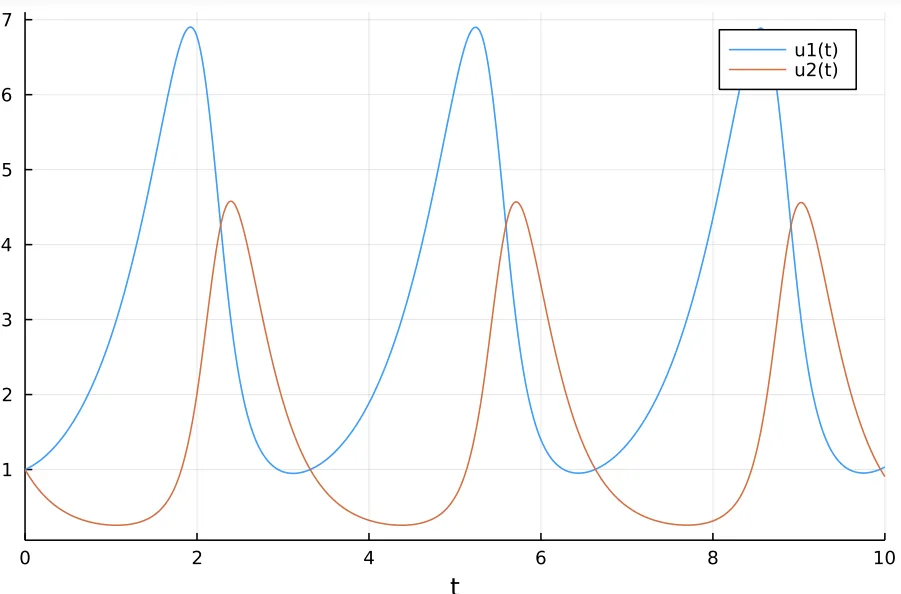

To be continued…

References

• Header Image
• [1] What’s New in the 2022 Gartner Hype Cycle for Emerging Technologies. (2022). Retrieved 10 September 2022, from https://www.gartner.com/en/articles/what-s-new-in-the-2022-gartner-hype-cycle-for-emerging-technologies
• [2] Mooij, J., Janzing, D., & Schölkopf, B. (2013). From Ordinary Differential Equations to Structural Causal Models: the deterministic case. Retrieved 10 September 2022, from https://arxiv.org/abs/1304.7920