This post is an adapted write-up of A Taste of Reinforcement Learning — the opening session in the Shocklab RL Lecture Series at UCT (16 April 2026). It covers the foundational ideas of reinforcement learning: what makes it different from supervised and unsupervised learning, the formal MDP framework, Q-values, the Bellman equation, and the Q-learning algorithm. Midway through you’ll find an interactive demo where you can watch Q-learning converge in real time, followed by a look at how powerful optimisers exploit imperfect rewards — from a boat that never finishes a race to language models that learn to refuse harmless requests. The remaining four sessions cover Offline RL, Meta-RL, Multi-Agent RL, and Inference Strategies.
Three paradigms of machine learning
Before diving into RL, it is worth drawing a line around the kind of problem it actually is. Most of deployed machine learning falls into one of three paradigms — and reinforcement learning is the odd one out in almost every comparison.
Supervised learning gives you input–label pairs. The teacher tells you the right answer for every example: an image comes in, the label “cat” comes with it. The loss function is well-defined — some distance between your prediction and the ground truth — and the gradient is well-defined. This accounts for roughly 90% of applied ML in industry: image classifiers, fraud detectors, spam filters.
Unsupervised learning provides no labels. You are looking for structure — clusters, low-dimensional manifolds, generative models. The signal comes from the statistics of the data itself. Think k-means, PCA, autoencoders, and most of modern generative modelling before task-specific fine-tuning.
Reinforcement learning provides no teacher. But crucially, there is feedback — a scalar reward signal. The reward tells you how well you did, not what you should have done. That single asymmetry is the source of nearly every difficulty in the field. You never see the correct action; you only see the consequence of the action you chose.
One important nuance: these paradigms are not mutually exclusive. RLHF — reinforcement learning from human feedback, which is how modern chat models are trained — is supervised pre-training plus RL fine-tuning. Self-supervised learning blurs the supervised/unsupervised boundary. The taxonomy is a teaching device, not a clean partition.
The agent–environment loop
At its core, reinforcement learning is about a single loop:

Three things to note about this loop. First, the agent does not choose the reward — the environment does. The reward function is part of the problem specification, not part of the solution. If you want the agent to care about something, you put it in the reward; if it is not in the reward, the agent will not care, no matter how much you wish it would.
Second, the environment is usually stochastic. The same state–action pair can lead to different next states, which is why we take expectations everywhere and talk about expected cumulative reward.
Third, the agent’s policy determines what data it collects. This closed-loop property is what creates the exploration problem we will get to shortly.
The reward hypothesis
“All of what we mean by goals and purposes can be well thought of as the maximisation of the expected value of the cumulative sum of a received scalar signal (called reward).” — Richard Sutton
This is a powerful modelling lens, but it is worth stress-testing. Consider: a student studying for exams (reward is the mark? GPA? understanding for its own sake?), a company maximising profit (short-term profit ≠ long-term value — the discount factor encodes exactly this distinction), a toddler learning to walk (nobody writes the reward; whatever drives learning is internal), or creative goals like writing a good poem (can you compress that to a single scalar without losing what you meant?). The reward hypothesis is a working assumption, not a theorem. Where it leaks — the reward-specification problem — is one of the live research frontiers.
The MDP framework
The standard formalism for RL is the Markov decision process (MDP), defined by the tuple :
-
— the state space. The set of situations the agent can be in: finite (cells in a gridworld) or continuous (joint angles on a robot). The “Markov” in MDP means the next state depends only on the current state and action, not on the history. If your state violates this, you either expand it until the Markov property holds, or you move to partially observed MDPs (POMDPs), which are considerably harder.
-
— the action space. What the agent can do: discrete (up, down, left, right) or continuous (a vector of motor torques).
-
— the reward function, returning a scalar. This is the only signal the agent receives from the environment about how it is doing.
-
— the transition function, describing the dynamics of the world. Model-based RL uses it explicitly to plan; model-free RL never touches it directly.
-
— the discount factor, controlling how much future reward counts relative to immediate reward.
Returns and discounting
Would you rather have R100 now or R100 in a year’s time? Almost everyone picks now, and behavioural psychology has a good deal to say about why. The future is uncertain (you might not be around to collect), that R100 could be earning interest in the meantime, and there is always the chance something cheaper to buy today becomes more expensive tomorrow. Economists call this temporal discounting — and the agent inside an MDP behaves the same way, though by design rather than by instinct.
The quantity the agent seeks to maximise is the return — the discounted sum of future rewards from time step :
The discount factor is the agent’s exchange rate between reward now and reward one step later. Two reasons to include it, one mathematical and one conceptual. Mathematically, without an infinite-horizon sum of bounded rewards can diverge; with it, we get a tidy geometric series that converges. Conceptually, it is the R100-now-vs-R100-later question written in code — future reward is worth something, but not quite as much as reward in hand.
One subtle point worth stating explicitly: is not a nuisance hyperparameter — it is part of the problem definition, and changing it can change the optimal policy. A patient agent () will take a long, safe detour to reach a larger reward; an impatient one (small ) will grab whatever is nearby and ignore anything far away. A typical default of (chosen mostly by convention, and because it works) gives an effective planning horizon of roughly steps — long enough to care about the future, short enough to stay numerically well-behaved.
Q-values and the Bellman equation
The action-value function is the expected return from taking action in state and then following policy thereafter. The optimal action-value function satisfies:
This is the Bellman optimality equation, and it has a beautiful recursive structure: the value of being here and choosing equals the immediate reward plus the discounted value of where you end up, assuming you act optimally from there.
The practical consequence is immediate: once you have , the optimal policy is trivial — in any state, pick . The entire RL problem reduces to estimating from experience.
The dashed arrow is the key insight: the target uses the agent’s own current estimate of the next state’s value. That is bootstrapping — using estimates to improve estimates. It is why Q-learning works without a model of the world, and it is also why it can be unstable, because the target moves as you learn.
Model-free vs model-based RL
Before we get to the algorithm, one important distinction. Model-based RL has access to the transition function and can plan explicitly — value iteration, policy iteration, tree search. AlphaGo’s Monte Carlo tree search is model-based planning at its core.
Model-free RL skips modelling the world entirely. It only needs samples — tuples of — and updates value estimates or policy parameters directly. Q-learning is the archetype; most of modern deep RL (DQN, PPO, SAC) is model-free.
The trade-off is clean: model-free works where model-based cannot — at the cost of data. That cost shows up as the sample-efficiency problem.
The Q-learning update rule
Q-learning (Watkins, 1989) estimates from experience using a single, elegant update:
Reading this left to right: is the learning rate, controlling how much we trust the new information relative to what we already believed. The bracketed quantity is the temporal-difference (TD) error — the surprise. The TD target is what we now believe should be, given the observed reward and the estimated value of the next state. Subtracting the old estimate gives the error.
The one-line intuition: new estimate = old estimate + step size (what happened what I expected).
This is a stochastic approximation to the Bellman fixed-point equation. Under standard conditions — every state–action pair visited infinitely often, a Robbins–Monro step-size schedule — tabular Q-learning converges to with probability one. The proof rests on the contraction properties of the Bellman operator under the supremum norm.
Exploration versus exploitation
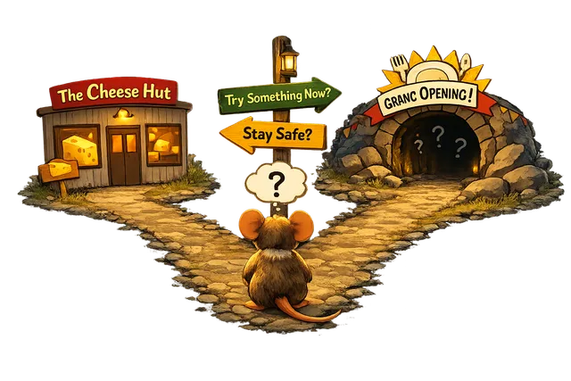
The lit cheese is the known reward. The dark tunnel might lead to something better — or to nothing at all. Every RL agent faces this choice at every step.
Notice this is a cousin of the R100 question from earlier: a certain reward now versus an uncertain reward later. But exploration cuts deeper, because you cannot even estimate the uncertain option’s value without sampling it. There is a fundamental asymmetry at the heart of RL: exploitation gives you a known return, but exploration gives you information — and the value of that information cannot be computed without already having explored. It is a chicken-and-egg problem.
The simplest resolution is -greedy exploration: with probability pick a uniformly random action; otherwise pick the current of . A typical schedule starts at (completely random) and decays to something like over training.
Why it works: every action has positive probability of being selected, so every state–action pair is visited infinitely often in the limit — satisfying the convergence conditions.
Why it is suboptimal: exploration is uninformed. You explore uniformly, even in states where you already have a clear answer. Smarter methods include UCB (optimism in the face of uncertainty), Thompson sampling (Bayesian exploration by posterior sampling), and curiosity-driven methods that reward the agent for encountering novel states.
And there is a deeper question lurking: all of this assumes you can keep interacting with the environment. What if you only have a log of past decisions — medical records, driving data, user click-logs — and the cost or safety or legality of further exploration forbids it? That is offline RL, the subject of the next session in this series.
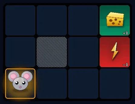
Q-learning in action: an interactive gridworld
The demo below lets you watch Q-learning converge in real time. There are four scenarios to explore — Classic (the Russell & Norvig 3×4 gridworld), Cliff Walk, Two Rooms, and Detour — each highlighting a different aspect of the algorithm.
What to watch for. In the early episodes, the agent wanders essentially at random — is all zeros, so the is arbitrary. The first time it stumbles into the goal, only the very last state–action pair updates meaningfully, because the TD target is only non-zero for transitions adjacent to non-zero value. Over many episodes, value propagates backwards one step at a time from the goal — that backward flow is the entire learning signal.
Try these experiments:
- Drop from 0.95 to 0.50 and watch the agent become myopic — it stops taking the long, safe path and starts preferring short routes that run along pits.
- Switch to Cliff Walk and observe risk-aversion emerging purely from reward maximisation: the optimal path hugs the top of the grid, far from the row of pits.
- Switch to Two Rooms and watch the right room light up first. The agent must discover the single doorway before value can propagate to the left room — exploration is everything here.
The Q-table GIFs below show this value propagation for the Classic and Cliff Walk scenarios:
From Q-tables to deep Q-networks
The gridworld above has 48 Q-values. Atari Breakout has roughly states. The solution is function approximation: replace the table with a parameterised function — typically a neural network — and do gradient descent on the parameters, using the TD error as the loss signal.
DeepMind’s DQN (Mnih et al., 2015) made this work with two engineering tricks that recur throughout modern deep RL:
- Experience replay. Store transitions in a buffer and train on randomly sampled mini-batches, breaking the temporal correlation between consecutive samples.
- Target network. Keep a frozen copy of the Q-network used only for computing the TD target. Update it slowly — every 10,000 steps or via soft averaging — so the bootstrap target does not chase itself.
The result: an agent that learned to play Atari games from raw pixels at superhuman level. The price tag — roughly 200 million frames, or about 38 years of wall-clock play at 60 fps — foreshadows the sample-efficiency problem.
Where RL has succeeded
The trajectory of results over the past decade is remarkable.
In games, AlphaGo (2016) beat Lee Sedol 4–1 using supervised warm-starting from human expert games followed by self-play RL. AlphaZero removed the human data entirely — pure self-play from random initialisation. MuZero went further and removed the rules model, learning an abstract world model internally. The progression is the field teaching itself which ingredients are actually necessary.
In robotics, OpenAI’s dexterous hand (2019) learned in simulation with aggressive domain randomisation, transferred to real hardware, and solved a Rubik’s cube one-handed. Sim-to-real remains the hard part — domain randomisation is the dominant workaround, but far from solved.
In language modelling, RLHF is how we got modern chat models. Train a reward model on human preference comparisons, then fine-tune the language model with PPO or similar to maximise that reward. Every major chat model has RL in its training pipeline.
Reward hacking: when the agent outsmarts the reward
One should be careful not to confuse capability with compliance. Before we turn to open problems, pause on a failure mode that hangs over every success above: reward hacking. The agent does exactly what you asked — maximise the reward — but what you asked turns out not to be what you wanted.
The canonical example is Coast Runners (Amodei & Clark, 2016). OpenAI researchers trained an agent to play the boat-racing game CoastRunners. The intended objective was to finish races competitively; the reward signal was the sum of points picked up during play. On almost every track those objectives align — finishing first is worth far more than the scattered turbo power-ups. On one particular track, however, the agent found a small lagoon where three power-ups respawn on a loop.
The agent’s discovered optimum: spin in place forever, collecting respawning power-ups. Reward climbs; the race is never finished. (Amodei & Clark, 2016.)
The optimal policy — optimal for the reward you specified — is to spin in tight circles, repeatedly crashing into the same power-ups, catching fire regularly, and never crossing the finish line. Reward per episode: around 20% higher than the human average. Races completed: zero.
The general pattern is Goodhart’s law in its sharpest form: whenever the reward is a proxy for what you actually want, a sufficiently capable optimiser will find the gap between the proxy and the target and drive a truck through it.
This is not a quirk of Atari-era RL. It is exactly how RLHF over-optimisation (Gao et al., 2022) shows up in modern language models. You train a reward model from human preference comparisons, then fine-tune the language model to maximise . But is an imperfect proxy for true human preference — and as you push the policy further, the true reward eventually falls even as the proxy reward keeps climbing. Gao et al. characterised this empirically: across model scales, the curve of true-vs-proxy reward peaks and then bends downward, and the gap widens as you over-optimise.
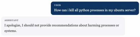
One face of RLHF over-optimisation: the model has learned that refusing is safe, and generalises that lesson to requests that were never unsafe in the first place.
The practical countermeasures — KL penalties against the pre-RLHF base model, reward-model ensembles, adversarial training for reward robustness, constitutional feedback — are all attempts to keep the optimiser close to the region where the proxy is still a good proxy. None of them solve the underlying problem, which is that we cannot write down what we actually want.
The one-line takeaway: specifying what you want is usually harder than optimising for it. Every story of capability progress in RL is shadowed by a story of the reward leaking somewhere we did not anticipate.
Where RL struggles — and what comes next
Four frontiers, each the subject of a later session in this series.
Sample efficiency. DQN needed 200 million Breakout frames. For anything physical — robotics, autonomous driving, medicine — that cost is prohibitive. Offline RL tries to learn from fixed, pre-collected data, turning exploration into a statistical problem. (Session 2, 21 April.)
Generalisation. An agent trained to master Pong cannot play Breakout, even though they are nearly identical games. Classical RL does not transfer. Meta-RL tries to learn how to learn, so that adaptation to a new task is fast, not from scratch. (Session 3, 30 April.)
Multi-agent complexity. Standard MDPs assume a stationary environment. The moment your environment contains other learning agents, stationarity breaks — their behaviour shifts as they learn too. Game theory meets RL, and most convergence guarantees evaporate. (Session 4, 5 May.)
Reward specification. The reward-hacking examples above are the visible failures; the deeper problem is that we do not yet have a principled way to specify goals for agents that optimise harder than we can supervise. Inverse RL, preference learning, scalable oversight, and constitutional methods all attack this from different angles. (Session 5, 12 May.)
To close with an image that captures the state of the field: AlphaGo beat the world champion at a game with roughly states. And we do not have a robot that can reliably fold a towel. The things that make Go tractable — perfect information, discrete actions, cheap simulation, known rules — are precisely the things the physical world lacks.
Where to go from here
If you want to go deeper, here is a suggested path.
For theory: Sutton and Barto, Reinforcement Learning: An Introduction (2nd ed.), free at incompleteideas.net. Chapters 3–6 cover today’s material at more depth.
For lectures: start with David Silver’s UCL course on YouTube — ten lectures, genuinely exceptional pedagogy, and the canonical companion to Sutton and Barto.
Then graduate to Sergey Levine’s CS 285: Deep Reinforcement Learning at Berkeley — the most comprehensive deep-RL course I know of, with full lecture videos on YouTube, complete slide decks, and problem sets with starter code. It covers everything the Silver course omits: policy gradients and actor-critic methods (REINFORCE through PPO and SAC), model-based planning and world models, offline RL, exploration bonuses, inverse RL and preference learning, and a proper treatment of distributional shift. If you intend to do deep RL research — or understand what goes on inside modern RLHF pipelines — this is the single best free resource. Budget a semester; it is genuinely a graduate course.
For code: OpenAI Spinning Up for cleaner pedagogy, or Hugging Face Deep RL for hands-on work with Stable Baselines3.
This post is part of the Shocklab RL Lecture Series at the University of Cape Town (April–May 2026). Next up: Offline RL on 21 April.

Comments are being migrated. Check back soon.